2 Probability Spaces and Random Variables
2.1 Probability Spaces
2.1.1 Definition
Let \(\Omega\) be a set and let \(\mathcal{P}(\Omega)\) be its power set, i.e. the family \(\left\{A\colon A\subset \Omega\right\}\).
Definition 2.1 A family of sets \(\mathscr{F}\subset \mathcal{P}\left(\Omega\right)\) is called a \(\sigma\)-algebra if it has the following properties:
\(\Omega\in\mathscr{F}\) and \(\emptyset\in\mathscr{F}\).
If \(A\in\mathscr{F}\) then \(A^c\in\mathscr{F}\).
If \((A_n)_{n\in\mathbb{N}}\subset\mathscr{F}\) is a countable collection of subsets in \(\mathscr{F}\), then \[\bigcup_{n=1}^\infty A_n\in\mathscr{F}.\] I.e. \(\mathscr{F}\) is closed under countable unions.
The pair \((\Omega,\mathscr{F})\) is called a measurable space.
Definition 2.2 Let \((\Omega,\mathscr{F})\) be a measurable space. A function \[\mathbb{P}\colon \mathscr{F}\to \mathbb{R}^+\] is called a probability measure if it satisfies the following properties:
\(\mathbb{P}(\Omega) = 1\) and \(\mathbb{P}(\emptyset)=0\).
\(\mathbb{P}(A)\geq 0\) for all \(A\in\mathscr{F}\).
- If \((A_n)_n\subset \mathscr{F}\) is a countable collection of pairwise disjoint sets, i.e. \[ A_i \bigcap A_j = \emptyset \quad \forall i\neq j, \] then \[ \mathbb{P}\left(\bigcup_n A_n\right) = \sum_n \mathbb{P}(A_n). \] The triplet \((\Omega,\mathscr{F},\mathbb{P})\) is called a probability space.
2.1.2 First Examples
Example 2.1 Set
- \(\Omega=[0,1]\),
- \(\mathscr{F}=\mathscr{B}([0,1])\) (safely ignore), and
- \(\mathbb{P}(A)=length(A)\)
- E.g. If \(A=[a,b]\) then \(\mathbb{P}(A)=b-a\)
Example 2.2 Set
- \(\Omega=[0,1]^n\),
- \(\mathscr{F}=\mathscr{B}([0,1]^n)\) (safely ignore), and
- \(\mathbb{P}(A)=volume(A)\),
- E.g. If \(n=2\) and \(A=[a,b]\times[c,d]\) then \(\mathbb{P}(A)=(b-a)(d-c)\).
- E.g.
In this case \(\mathbb{P}\left(A\right)=\sum_{n=1}^\infty \left(\frac{1}{2^2}\right)^n = 1/3\).
2.1.3 Important Examples
2.1.3.1 Probability Measures with Density on \(\mathbb{R}\) (or \(\mathbb{R}^+\), etc)
Definition 2.3 (Probability Measure with Density) Let \(f\colon D\subset\mathbb{R}\to \mathbb{R}^+\) be such that \(\int_D f(x)\hspace{3pt}dx = 1\). Such an \(f\) is called a density function on \(D\). Set
- \(\Omega=D\),
- \(\mathscr{F}=\mathscr{B}(D)\) (safely ignore), and
- \(\mathbb{P}(A)=\int_{A\cap D} f(x) \hspace{3pt}dx\)1
- E.g. If \(D=\mathbb{R}\) and \(A=[a,b]\) then \(\mathbb{P}(A)=\int_a^b f(x)\hspace{3pt}dx\).
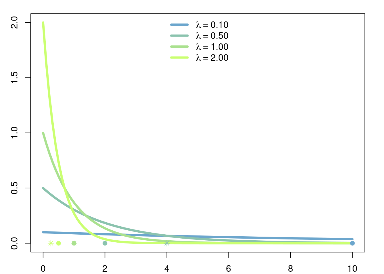
Example 2.3 (Exponential Measure) Let \(D=\mathbb{R}^+\). For any \(\lambda>0\) set \[f(x)= \lambda e^{-\lambda x},\] \(f\) satisfies \[\int_0^\infty f(x) \hspace{3pt}dx=\int_0^\infty \lambda e^{-\lambda x} \hspace{3pt}dx= 1.\]
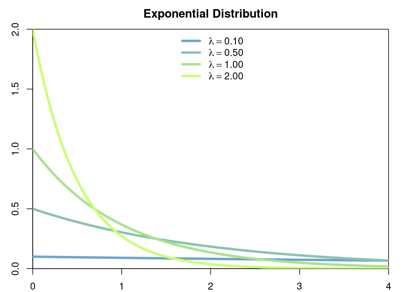
Thus we may define a continuous probability measure \(\mathbb{P}\) on \(\mathbb{R}^+\) which satisfies, for example \[\mathbb{P}([a,\infty])=\int_a^\infty \lambda e^{-\lambda x}\hspace{3pt}dx=e^{-\lambda a}.\]
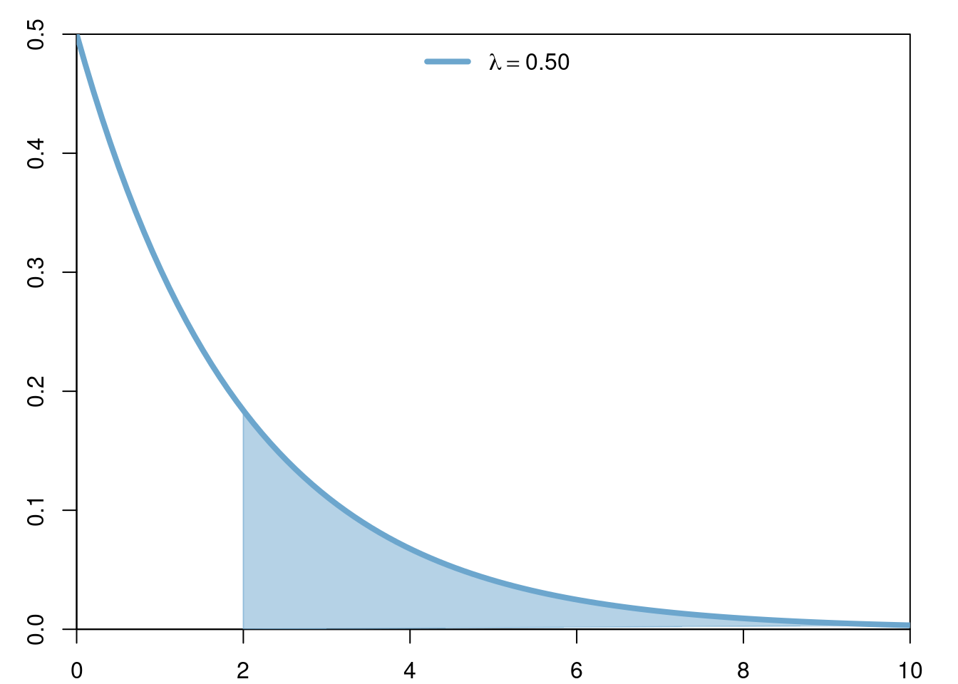
In this case \(\mathbb{P}[(2,\infty)]=\int_2^\infty 0.5e^{-0.5x}\hspace{3pt}dx = e^{-1}\).
2.1.3.2 Discrete Probability Measures on \(\mathbb{R}\) (or \(\mathbb{N}\), etc)
Definition 2.4 (Discrete Probability Measure) Let \((a_n)_n\subset\mathbb{R}\) be a countable collection of points in \(\mathbb{R}\) (resp. \(\mathbb{N}\), etc), and let \((p_n)_n\subset [0,1]\) be such that \[\sum_n p_n = 1.\] Set
- \(\Omega=\mathbb{R}\),
- \(\mathscr{F}=\mathscr{B}(\mathbb{R})\) (safely ignore),
- \[\mathbb{P}(A)=\sum_{n\colon a_n\in A}p_n \]
- E.g. If \(a_n=n\) for \(1\leq n \leq N\) and \(p_n=1/N\), then \(\mathbb{P}(\{1,2\}) = \frac{1}{N} + \frac{1}{N}=\frac{2}{N}\)
Example 2.4 (Geometric Measure) Let \(a_0=0, a_1=1, a_2=2, \dots\) and fix any \(p\in[0,1];\) define \(p_n=p^n(1-p)\) for \(n\in\{0,1,\dots\}\) and note that they satisfy2 \[ \begin{aligned} \sum_{n=0}^\infty p^n(1-p) &= (1-p)\sum_{n=0}^\infty p^n \\ &= \frac{1-p}{1-p} \\ &= 1. \end{aligned} \]
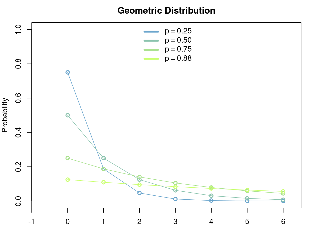
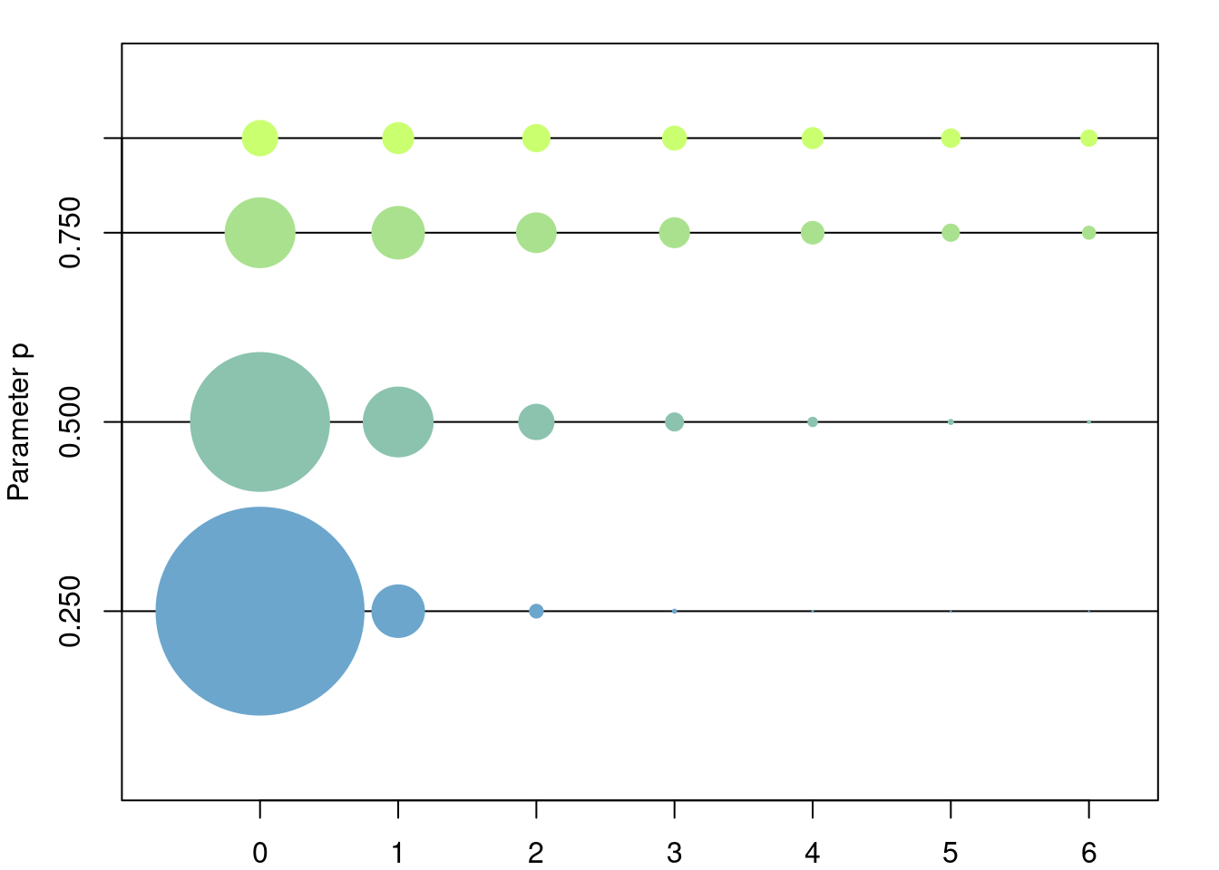
Thus we may define a probability measure \(\mathbb{P}\) on \(\mathbb{N}\) (or on \(\mathbb{R}\)). For any \(k\in \mathbb{N}\) this probability measure evaluated on the set \(\{0,\dots,k\}\) gives \[ \begin{aligned} \mathbb{P}(\{0,\dots,k\}) &= (1-p)\sum_{n=0}^k p^n \\ &= (1-p)\frac{1-p^{k+1}}{1-p}\\ &=1-p^{k+1}. \end{aligned} \]
2.1.4 Properties of Probability Measures
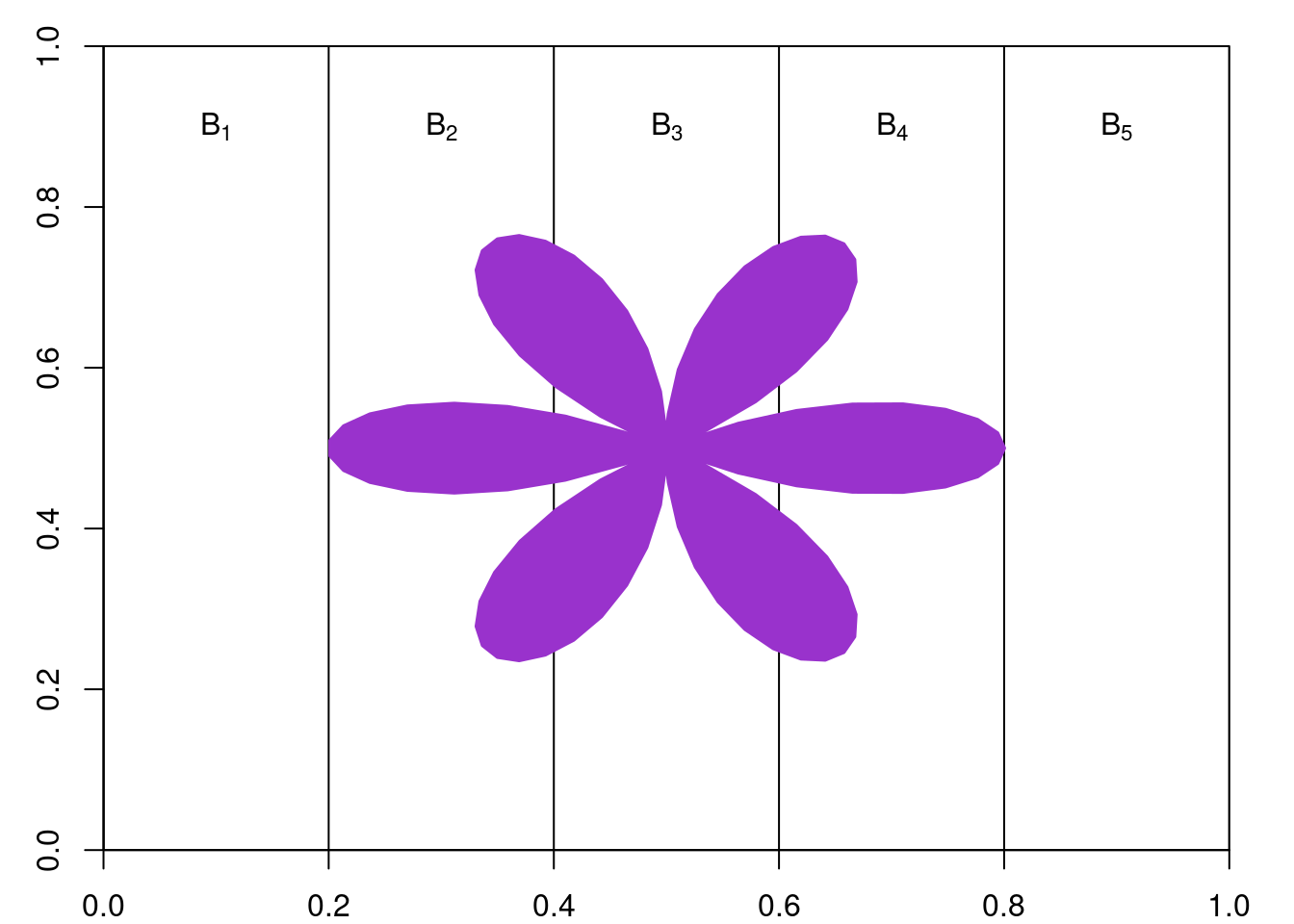
Theorem 2.1 Let \((B_n)_n\subset\mathscr{F}\) be a partition of \(\Omega\), i.e.
- \(\bigcup_n B_n = \Omega\), and
- \(B_n \bigcap B_m = \emptyset \quad \forall n\neq m\),
Theorem 2.2 Let \((\Omega,\mathscr{F}, \mathbb{P})\) be a probability space. The following equalities hold.
If \((A_n)_{n\in\mathbb{N}}\subset \mathscr{F}\) and \[ A_{n}\subset A_{n+1} \quad\forall n\in\mathbb{N}, \] then \[ \mathbb{P}\left(\bigcup_{n} A_n\right) = \lim_{n\to\infty} \mathbb{P}\left(A_n\right). \]
- If \((A_n)_{n\in\mathbb{N}}\subset \mathscr{F}\) and \[ A_{n+1}\subset A_{n} \quad\forall n\in\mathbb{N}, \] then \[ \mathbb{P}\left(\bigcap_{n} A_n\right) = \lim_{n\to\infty} \mathbb{P}\left(A_n\right). \]
2.2 Random Elements
2.2.1 Single Random Variables
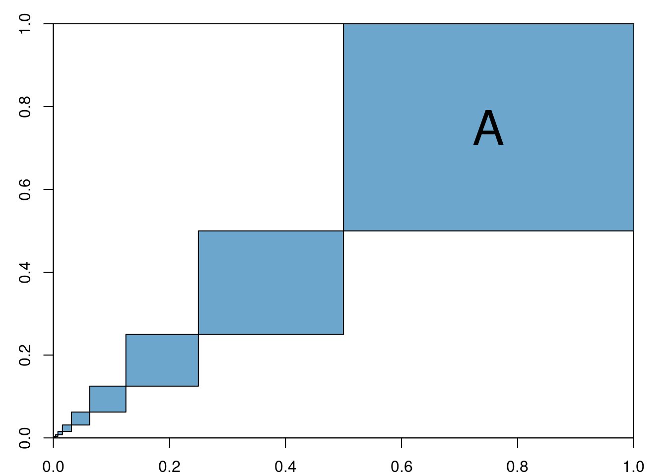
Example 2.5 Recall Example 2.1 where \(\Omega = [0,1]\) and \(\mathbb{P}(A)=length(A)\). Let \(N\in\mathbb{N}\) and define the function \(X\colon [0,1]\to\mathbb{N}\) given by
\[ X(\omega):=n \quad \text{ if }\quad \frac{n-1}{N} \leq \omega \leq \frac{n}{N}, \quad n\in\{1,\dots,N\}. \]
In this case \(X\) has the (discrete) uniform distribution on the set \(\{1,\dots, N\}\) since all the points have the same probability measure, that is \[ \forall i,j\in\{1, \dots, N\},\quad\mathbb{P}(X=i)=\frac{1}{N}=\mathbb{P}(X=j). \]In this course we will only deal with distributions of the forms presented in Subsection 2.1.3.
Definition 2.7 (Continuous and Discrete Random Variables.) Let \(X\) be a random variable.
\(X\) is a continuous random variable, or its distribution is said to be continuous, if \[ \mathbb{P}(X\in A) = \int_A f_X(x) \hspace{3pt}dx \] for some density function \(f_X\).
- \(X\) is a discrete random variable, or its distribution is said to be discrete, if \[ \mathbb{P}(X\in A) = \sum_{a_n\in A} p_n \] where \((a_n)_n\) is a countable collection of points in \(\mathbb{R}\) and \((p_n)_n\) is a collection of probabilities that sum to 1.
2.2.2 Random Vectors
In general we often want to be able to deal with multiple random variables at once, this is why at this point it is useful to think of an abstract probability space \((\Omega, \mathscr{F}, \mathbb{P})\) and simply assume that it is rich enough so that we can define/asssure the existence of different random variables with any properties that might interest us. In fact we often make no mention at all of the underlying probability space \((\Omega, \mathscr{F}, \mathbb{P})\) and simply talk about random variables, random vectors, etc, and their distributions.
Definition 2.8 (Random Vectors) Let \((\Omega,\mathscr{F},\mathbb{P})\) be a probability space. A function of the form \[ \begin{aligned} \bar{X}\colon \Omega &\to \mathbb{R}^n \\ \omega &\mapsto \bar{X}(\omega)=(X_1(\omega),\cdots,X_n(\omega)) \end{aligned} \] is called a random vector.
Random vectors induce a probability measure on \(\mathbb{R}^n\) by considering, for any \(A\in\mathscr{B}(\mathbb{R}^n)\) \[ A\mapsto \mathbb{P}(\bar{X}\in A) = \mathbb{P}\left(\left\{\omega\in\Omega\colon \bar{X}(\omega)\in A \right\}\right). \] The probability measure induced by a random vector is called its distribution.Similarly as in the case of single random varibles, we may consider continuous random vectors whose distribution is given by a density function \(f_{\bar{X}}\colon \mathbb{R}^n \to \mathbb{R}^+\), and discrete random vectors whose distribution is given by a countable collection of points and probabilities \((a_n)_n\) and \((p_n)_n\).
Example 2.6 (Continuous Random Vector Density) Let \(f_1,\dots,f_n\) be \(n\) density functions on \(\mathbb{R}\). Define a density function \(f\) on \(\mathbb{R}^n\) as \[ f(x_1,\dots,x_n) = \prod_{k=1}^n f_k(x_k), \] and consider a random vector \(\bar{X}=(X_1,\dots,X_n)\) with density function \(f\).
In particular note that for any \(A_1,\dots,A_n\in\mathscr{B}(\mathbb{R})\) and \(A=A_1\times\dots\times A_n\) we have
\[ \begin{aligned} \mathbb{P}(\bar{X}\in A) &= \mathbb{P}\left(X_1\in A_1,\dots, X_n\in A_n\right) \\ &=\int_{A_1}\dots \int_{A_n} f(x_1, \dots, x_n) \hspace{3pt}dx_n \dots \hspace{3pt}dx_1 \\ &=\int_{A_1}\dots \int_{A_n} \prod_{k=1}^n f_k(x_k) \hspace{3pt}dx_n \dots \hspace{3pt}dx_1 \\ &=\prod_{k=1}^n \int_{A_k} f_k(x) \hspace{3pt}dx \\ &=\prod_{k=1}^n \mathbb{P}(X_k\in A). \end{aligned} \]
```
Example 2.7 (Random Parameter - Exponential Case) Recall the exponential distribution introduced in Example 2.3. Let \(f\) be a density function on \(\mathbb{R}^+\). Define the density \(g\colon (\mathbb{R}^+)^2\to\mathbb{R}\) as \[ g(\lambda, X) = \lambda e^{-\lambda x}f(\lambda). \]
Let \((\Lambda, X)\) be a random vector with density \(g\). The distribution of \(X\) can be interpreted algorithmically: 1) first choose a random parameter \(\Lambda\) according to the density \(f\), 2) then generate a random variable \(X\) that is exponentially distributed of parameter \(\Lambda\).2.3 Conditional Probability and Independence
2.3.1 Intuition
Let \((\Omega,\mathscr{F},\mathbb{P})\) be a probability space and let \(A\in\mathscr{F}\) be a set with positive measure, i.e. \[ \mathbb{P}\left(A\right)>0. \] Let \(B\in\mathscr{F}\) be another set. We would like to know what is the probability that \(B\) occurs given that we already know that \(A\) occurs. That is, we would like to know the updated probability of the event \(B\) after we weigh in the extra information that we know that \(A\) occurs. For example, if \(B\cap A=\emptyset\) then knowing that \(A\) occurs tells us that \(B\) does not occur so in this case \(\mathbb{P}(B\vert A) = 0\). In general we have the formula \[ \mathbb{P}\left(B\vert A\right) = \frac{\mathbb{P}(B \cap A)}{\mathbb{P}(A)} \] which follows from the reasoning that knowing that \(A\) occurs reduces our initial probability space \(\Omega\) to the set \(A\) which then becomes the new ‘total’ or ‘universe’ set, and in order to equip the space \(A\) with a probability measure we simply normalize our initial probability measure \(\mathbb{P}\) by the measure of the set \(A\), i.e. by \(\mathbb{P}(A)\).
Particularly, for random variables \(X\) and \(Y\) we find the conditional probability that \(X\in B\) given that we already know that \(Y\in A\) as \[ \mathbb{P}(X\in B \vert A\in A) = \frac{\mathbb{P}(X\in B, Y\in A)}{\mathbb{P}(Y\in A)}. \]
2.3.2 Discrete case
Let \(Y\) be a discrete random variable, and suppose that \(\mathbb{P}(Y = a)>0\). Then, for any \(B\in \mathscr{F}\) we have \[ \mathbb{P}(X\in B \vert Y=a) = \frac{\mathbb{P}(X\in B, Y = a)}{\mathbb{P}(Y=a)}. \] Compare this with the continuous case scenario. The following formula is often used when computing probabilities by first assuming that we know the value of the random variable \(Y\), thus computing \(\mathbb{P}(X\in B\vert Y = a)\), and then summing over the possible values for \(Y\). Indeed, let \((a_n)_{n}\) be the set of values for \(Y\), then
\[ \begin{aligned} \mathbb{P}\left(X \in B\right) &= \sum_{n}\mathbb{P}(X \in B, Y = a_n)\\ &= \sum_{n} \mathbb{P}(X\in B \vert Y = a_n) \mathbb{P}(Y = a_n). \end{aligned} \]
More generally we have
\[ \mathbb{P}\left(X \in B, Y\in A\right) = \sum_{n\colon a_n\in A} \mathbb{P}(X\in B \vert Y = a_n) \mathbb{P}(Y = a_n). \]
2.3.3 Continuous Case
Let \(Y\) be a continuous random variable, in which case we always have that, for any \(a\in\mathbb{R}\), \(\mathbb{P}(Y=a)=0\). In this case we cannot define a conditional probability given that \(Y=a\) as we did before (by simply normalizing with \(\mathbb{P}(Y=a)\)), but we can in fact define a conditional density function. So let \(X\) be another random variable and consider the random vector \((X,Y)\) with (joint) density function \(f_{X,Y}(x,y)\). For each fixed value of \(y\) define the conditional density function \(X\) given \(Y=y\) as \[ f_{X\vert Y}(x\vert y) = \frac{f(x,y)}{\int_{-\infty}^\infty f(x,y) dx } = \frac{f(x,y)}{f_Y(y)}, \] and define the conditional probability of \(X\in B\) given \(Y=y\) through the integral of the conditional density function:
\[ \mathbb{P}(X\in B\vert Y=y) = \int_B f_{X\vert Y}(x\vert y) dx. \]
Observe that
\[ f_{X,Y}(x,y) = f_{X\vert Y}(x\vert y)f_Y(y), \]
so that, for any \(B,A\in\Omega\),
\[ \begin{aligned} \mathbb{P}(X\in B, Y\in A) &= \int_A \int_B f_{X,Y}(x,y) dx dy \\ &=\int_A \int_B f_{X\vert Y}(x\vert y)f_Y(y) dx dy\\ &= \int_A \mathbb{P}(X\in B \vert Y = y)f_Y(y) dy. \end{aligned} \]
2.3.4 Independence
Compare this with the general formula \[ \mathbb{P}\left(A \bigcap B\right) = \mathbb{P}(A\vert B) \mathbb{P}(B) \] which is always true; observe that the definition of independence can be seen as the property that \[ \mathbb{P}(A\vert B) = \mathbb{P}(A), \] which says that having information about the event \(B\) does not provide us with any additional information about \(A\), and thus our ‘knowledge’ that \(A\) occurs (or may occur) remains the same.
The property in the definition of independence, i.e. that \(\mathbb{P}\left(X\in A \bigcap Y\in B\right) = \mathbb{P}(X\in A) \mathbb{P}(Y\in B)\), can be strengthen to \(\mathbb{P}\left(h(X)\in A \bigcap g(Y)\in B\right) = \mathbb{P}(h(X)\in A) \mathbb{P}(g(Y)\in B)\) for any pair of functions \(f\) and \(g\), and, furthermore, can be extended to a stronger property about expectations (see Theorem ?? below).
2.4 Cumulative Distribution Functions (CDFs)
2.4.1 Single Random Variables
a <- 0
b <- 3
x <- seq(a-2, b+2, length.out = 100)
par('plt' = c(0.08, 1-0.05, 0.08, 1-0.05), 'xaxs' = "r", 'yaxs' = "r")
plot(x = x, y = punif(x, min = a, max = b), type = "l", col = "skyblue3", lwd = 3)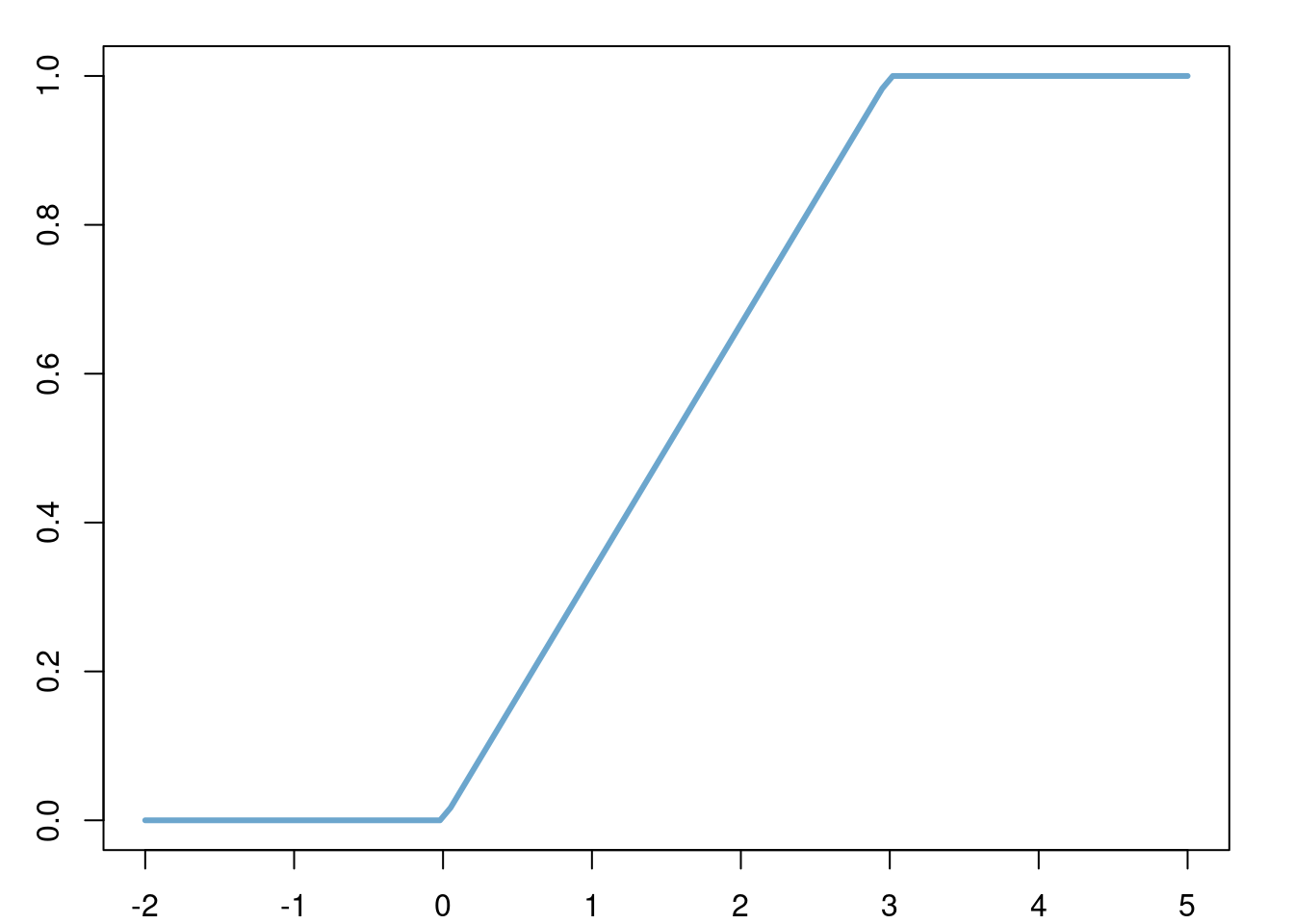
Exercise 2.7 Recall Example 2.4. Compute the CDF of the geometric distribution of parameter \(p\).
Exercise 2.8 Recall Example 2.3. Compute the CDF of the exponential distribution of parameter \(\lambda\).
p <- 0.75
x <- seq(-1, 6, length.out = 1000)
par('plt' = c(0.08, 1-0.05, 0.08, 1-0.05), 'xaxs' = "r", 'yaxs' = "r")
plot(x = x, y = pgeom(x, p = p), type = "p", col = "skyblue3", lwd = 1)
points(x = 0:5, y = pgeom(0:5, p = p), col = "red", lwd = 3, pch = 19)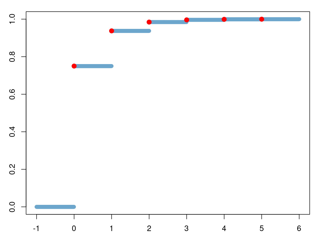 ```
```
lambda <- 5
x <- seq(0, 6, length.out = 1000)
par('plt' = c(0.08, 1-0.05, 0.08, 1-0.05), 'xaxs' = "r", 'yaxs' = "r")
plot(x = x, y = pexp(x, rate = lambda), type = "l", col = "skyblue3", lwd = 3)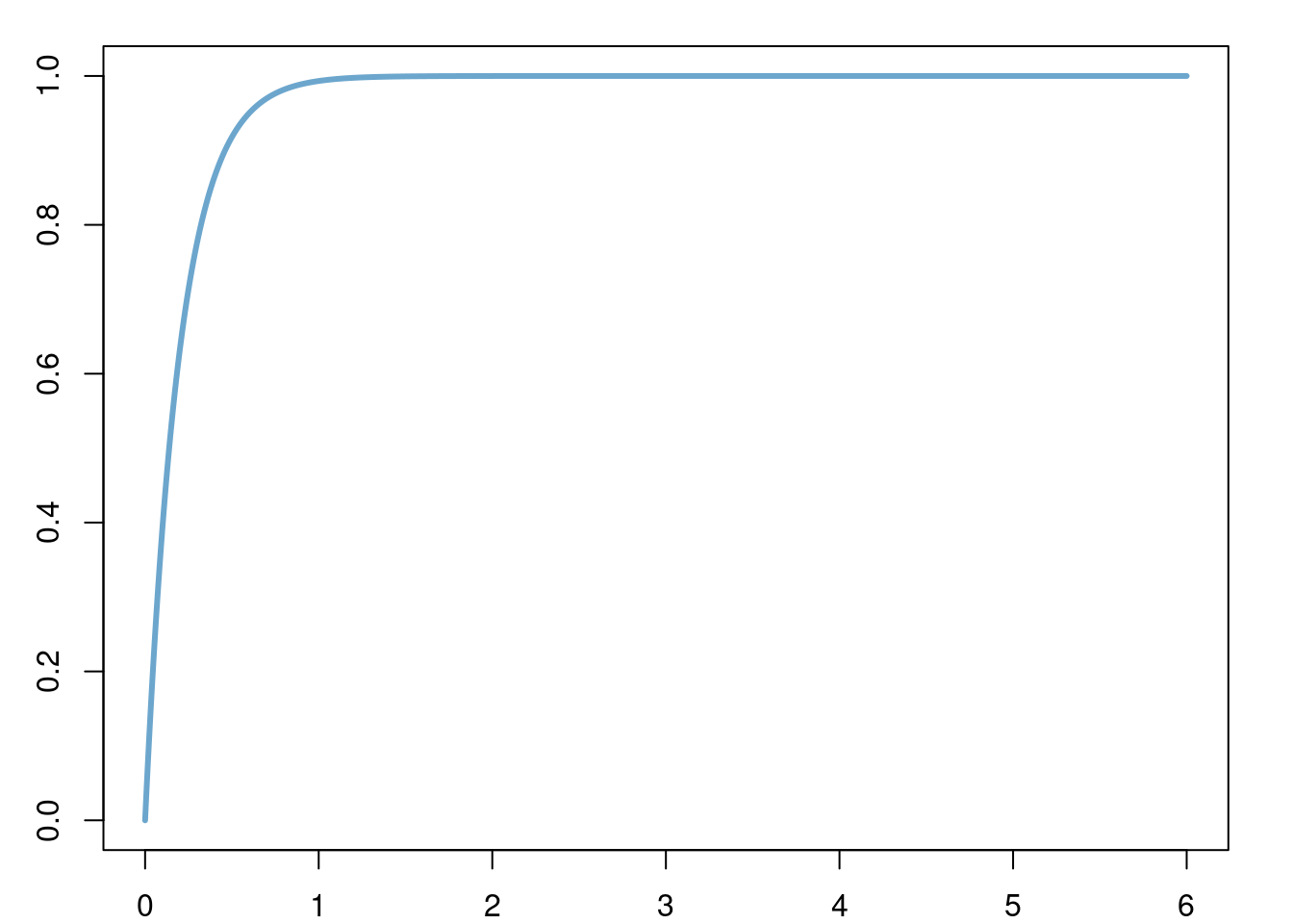
Theorem 2.4 (Properties of CDFs) A function \(F\) is a cumulative distribution function if and only if
- \(F(-\infty):=\lim_{x\to-\infty}F(x)=0\) and \(F(\infty):=\lim_{x\to\infty}F(x)=1\).
- \(F\) is right continuous, i.e. for all \(y\in\mathbb{R}\), \(\lim_{x\downarrow y} F(x) = F(y)\).
- \(F\) is non-decreasing, i.e. for all \(x<y\), \(F(x)\leq F(y)\).
Theorem 2.5 is often useful in determining the distribution of a function of a random variable, say \(h(X)\), by attempting to compute \[ \mathbb{P}(h(X) \leq x) \] for all \(x\).
Definition 2.15 (Continuous and Discrete Random Variables) Let \(X\) be random variable.
- \(X\) is a continuous continuous random varible if \(F_X\) is continuous.
- \(X\) is a discrete random variable if \(F_X\) is piecewise constant.
In this course we will assume that continuous random variables have a probability distribution with a density (recall Definition 2.3 ), or,
in other words, we will assume that for any continuous random variable \(X\) with CDF \(F_X\), we have \(F_X'=f_X\) for some
density function \(f_X\) and
\[
F_X(x) = \int_{-\infty}^x f_X(s) \hspace{3pt}ds.
\]
2.5 Expectations and Moments
2.5.1 Single Random Variables
Definition 2.16 (Expectation - Single Random Variables) Let \(X\) be a random variable, \(h\colon \mathbb{R}\to\mathbb{R}\) be a function, and consider the random variable \(h(X)\). We define the expected value of h(X), \(\mathbb{E}[h(X)]\) as:
if \(X\) is continuous with density \(f_X\), \(\mathbb{E}[h(X)]\) is the integral \[ \mathbb{E}\left[h(X)\right] :=\int_{-\infty}^\infty h(x)f_X(x)\hspace{3pt}dx. \]
if \(X\) is discrete and takes values \((a_n)_n\) with probabilities \((p_n)_n\) \(\mathbb{E}[h(X)]\) is the sum \[ \mathbb{E}\left[h(X)\right] :=\sum_{n} p_n h(a_n). \]
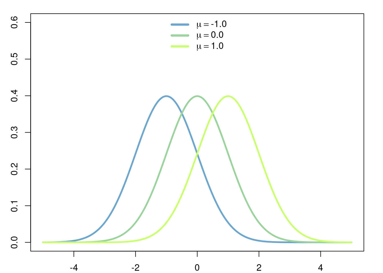
Example 2.13 (Mean of Normal Distribution) In this example we will assume the known fact that \[ \int_{-\infty}^\infty e^{-x^2} \hspace{3pt}dx = \sqrt{\pi}. \]
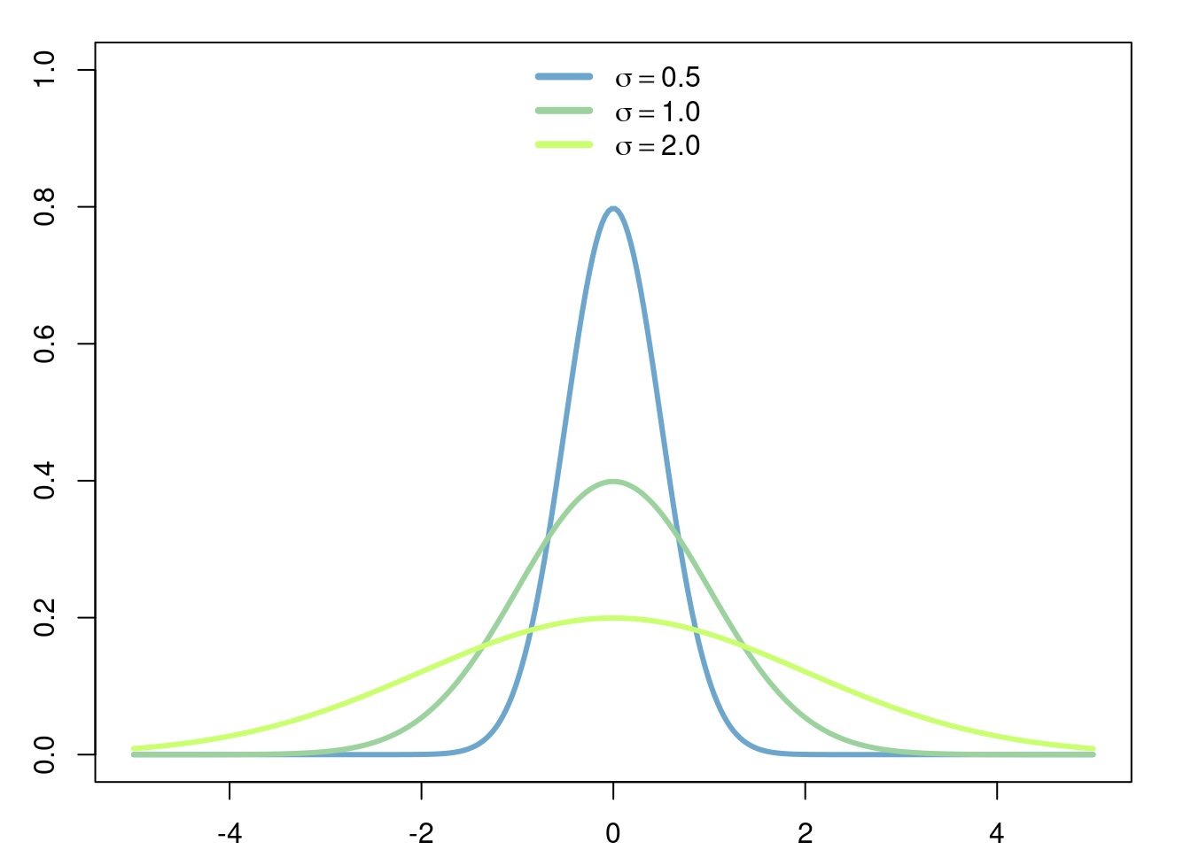
Let \(X\) be a random variable with density function \[ f(x) = \frac{e^{-\frac{(x-\mu)^2}{2\sigma^2}}}{\sigma\sqrt{2\pi}}. \]
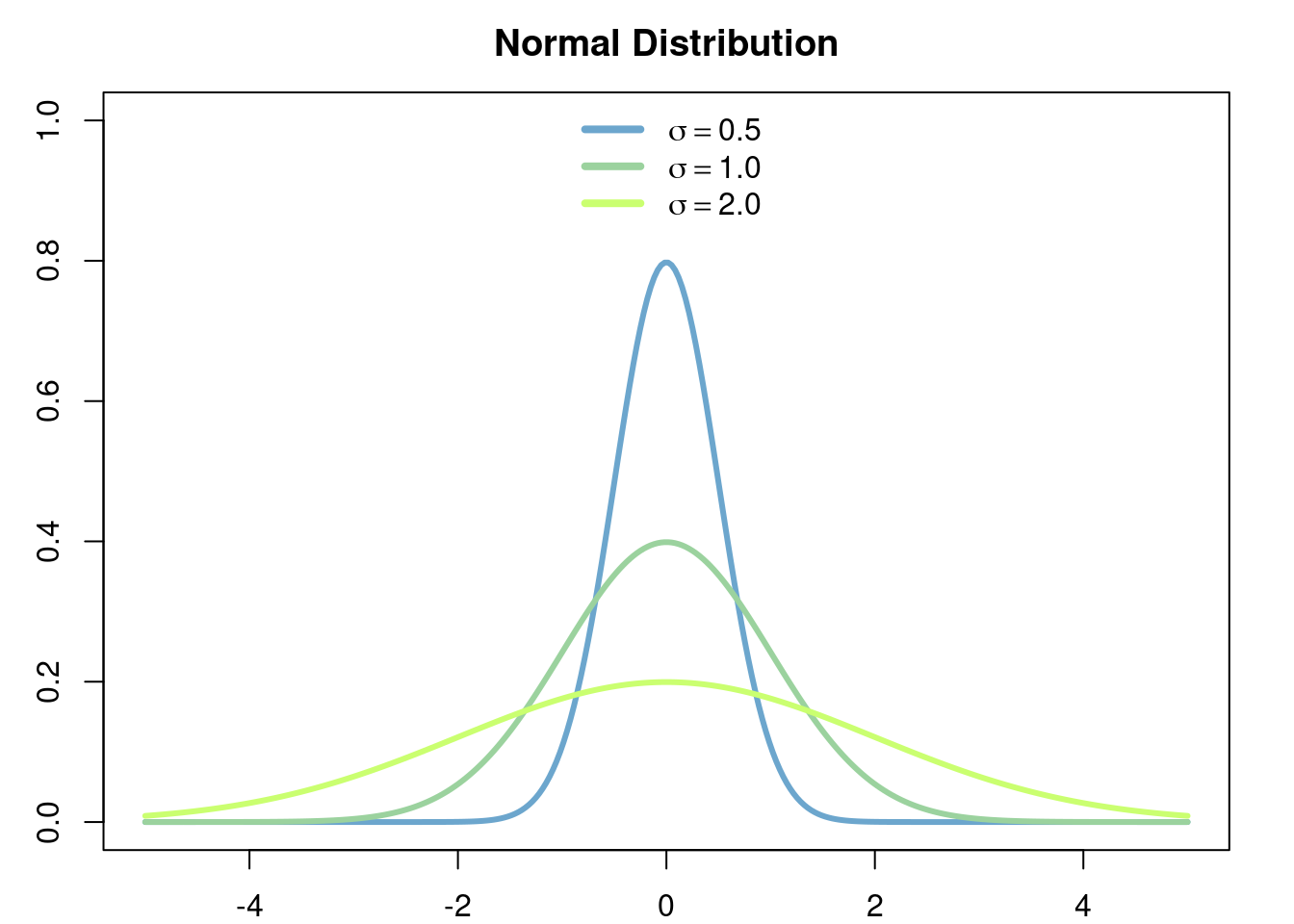
The distribution associated to this density function is called the normal distribution (with mean \(\mu\) and variance \(\sigma^2\)). Then the expected value (mean) of \(X\) is given by
\[ \begin{aligned} \mathbb{E}\left[X\right] &= \int_{-\infty}^\infty x \frac{e^{-\frac{(x-\mu)^2}{2\sigma^2}}}{\sigma\sqrt2\pi} \hspace{3pt}dx\\ &= \int_{-\infty}^\infty (\sigma\sqrt{2}y+\mu) \frac{e^{-y^2}}{\sigma\sqrt{2\pi}} \sigma\sqrt{2}\hspace{3pt}dy\\ &= \int_{-\infty}^\infty \sigma\sqrt2 y \frac{e^{-y^2}}{\sqrt{\pi}}\hspace{3pt}dx + \frac{\mu}{\sqrt\pi} \int_{-\infty}^\infty e^{-y^2}\hspace{3pt}dy. \end{aligned} \]
where we have used the change of variable \(y=\frac{x-\mu}{\sigma\sqrt{2}}\). Now observe that the function \(e^{-y^2}\) is symmetric around 0, therefore
\[ \int_{-\infty}^0 \sigma\sqrt2 y \frac{e^{-y^2}}{\sqrt{\pi}}\hspace{3pt}dx = - \int_0^\infty \sigma\sqrt2 y \frac{e^{-y^2}}{\sqrt{\pi}}\hspace{3pt}dx, \]
which implies
\[ \int_{-\infty}^\infty \sigma\sqrt2 y \frac{e^{-y^2}}{\sqrt{\pi}}\hspace{3pt}dx = 0. \]
Thus
\[ \mathbb{E}\left[X\right] = \mu. \]
Let \(\lambda > 0\). Let \(X\) be the discrete random variable with distribution given by \[ \mathbb{P}(X = n) = e^{-\lambda} \frac{\lambda^n}{n!},\quad \forall n\in\mathbb{Z}^+=\{0,1,2,\dots\} \]
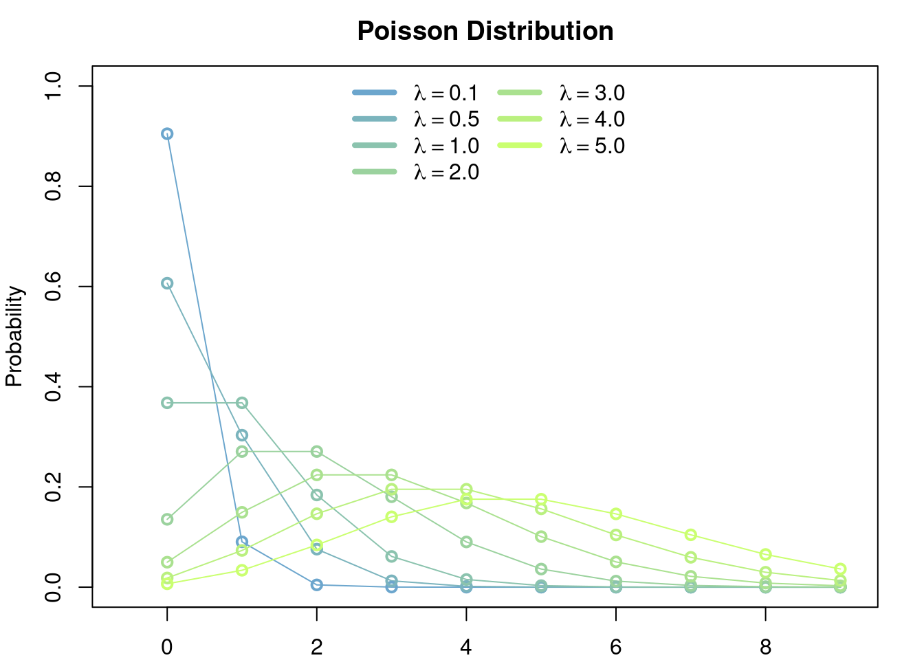
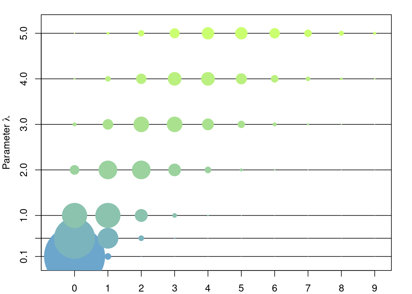
Exercise 2.10 Argue why this is a valid definition of a discrete random variable.
A random variable with the above distribution is called a Poisson random variable of parameter \(\lambda\). The expected value of \(X\) is given by \[ \begin{aligned} \mathbb{E}[X] &= e^{-\lambda}\sum_{n=0}^\infty n \frac{\lambda^n}{n!} \\ &= e^{-\lambda}\sum_{n=1}^\infty n \frac{\lambda^n}{n!} \\ &= \lambda e^{-\lambda}\sum_{n=0}^\infty \frac{\lambda^{n-1}}{(n-1)!}\\ &= \lambda \end{aligned} \]
Theorem 2.6 (Linearity of Expected Values) Let \(X\) and \(Y\) be two random variables. Then
\[\mathbb{E}[X + bY] = \mathbb{E}[X] + b\mathbb{E}[Y].\]
Exercise 2.15 (Variance of Exponential Distribution) Prove that if \(X\) is exponentially distributed with parameter \(\lambda>0\), then \[ \mathbb{Var}(X) = \frac{1}{\lambda^2}. \]
2.5.2 Random Vectors
Definition 2.19 (Expected Value - Random Vectors) Let \(X\) be a random variable, \(h\colon \mathbb{R}\to\mathbb{R}\) be a function, and consider the random variable \(h(X)\). We define the expected value of h(X), \(\mathbb{E}[h(X)]\) as:
if \(\bar{X}\) has density \(f_{\bar{X}}\) then \(\mathbb{E}[h(\bar{X})]\) is the multiple integral \[ \mathbb{E}\left[g(\bar{X})\right] :=\int_{-\infty}^\infty\dots \int_{-\infty}^\infty g(x_1,\dots,x_n)f_{\bar{X}}(x_1,\dots,x_n) \hspace{3pt}dx_1,\dots,x_n, \]
if \(\bar{X}\) is a discrete random vector taking values \((a_k)_k\subset\mathbb{R}^n\) with probabilities \((p_k)_k\), then, in the same way as in the single random variable case, \(\mathbb{E}[h(\bar{X})]\) is the sum \[ \mathbb{E}\left[g(\bar{X})\right] = \sum_{k} p_k g(a_k), \]
- if \(\bar{X}=(X_1,\dots,X_n)\) is such that some coordinates are discrete random variables and some are continuous random variables, then to compute \(\mathbb{E}[h(\bar{X})]\) we integrate or sum correspondingly.
Example 2.19 (Randomized Bernoulli) Recall the random vector \((\rho, X)\) of Example 2.8. Then \[ \mathbb{E}[X] = \int_0^1 (p\cdot 1 + (1-p)\cdot 0) f(p) \hspace{3pt}dp =\mathbb{E}[\rho]. \] Similarly \[ \mathbb{E}[X/\rho] = \int_0^1 \frac{(p\cdot 1 + (1-p)\cdot 0)}{p} f(p) \hspace{3pt}dp = 1. \]
Let \(f\colon \mathbb{R}\to\mathbb{R}\) be a function and \(A\subset \mathbb{R}\). Let \(\mathbb{1}_A\) be the indicator function of \(A\), i.e. the function \[ \mathbb{1}_A(x) \begin{cases} 1 & \text{ if } x\in A\\ 0 & \text{ otherwise}, \end{cases} \] then the integral of \(f\) on the set \(A\) is defined as \[ \int_A f(x)\hspace{3pt}dx = \int_{-\infty}^\infty \mathbb{1}_A(x)f(x) \hspace{3pt}dx. \] For example, if \(A=[a,b]\cup [c,d]\), then \[ \begin{aligned} \int_A f(x)\hspace{3pt}dx &= \int_{-\infty}^a 0 \hspace{3pt}dx + \int_a^b f(x) \hspace{3pt}dx + \int_b^c 0 \hspace{3pt}dx + \int_c^d f(x) \hspace{3pt}dx + \int_d^\infty 0\hspace{3pt}dx\\ &= \int_a^b f(x) \hspace{3pt}dx + \int_c^d f(x) \hspace{3pt}dx. \end{aligned} \]↩
Let \(p\in (0,1)\). Let \(S_N\) \[ \begin{aligned} S_N &:=\sum_{k=0}^N p^k\\ &= p^0 + p^1 + \dots + p^{N}, \end{aligned} \] \(S_N\) is the partial sum of \(p^k\) up to \(k=N\). We want to compute \[ S_\infty :=\sum_{k=0}^\infty p^k = \lim_{N\to\infty} S_N. \] Observe that \[ \begin{aligned} pS_N &= p \sum_{k=0}^N p^k \\ &= \sum_{k=0}^N p^{k+1} \\ &= p^1 + \dots + p^{N+1} \\ &= S_{N} + p^{N+1} - 1, \end{aligned} \] where we have used that \(p^0=1\) in the last equality. Rearranging terms we obtain \[ S_N = \frac{1-p^{N+1}}{1-p}; \] thus, since \(0<p<1\) which implies \(\lim_{N\to\infty} p^{N+1}=0\), we have \[ \sum_{k=0}^\infty p^k = \lim_{N\to\infty} S_N = \lim_{N\to\infty} \frac{1-p^{N+1}}{1-p} = \frac{1}{1-p}. \]↩
More formally, if \(X\) takes values in \(E_1\) and \(Y\) takes values in \(E_2\) (e.g. \(E_1\) and \(E_2\) may be \(\mathbb{R}^n\), \(n\in\mathbb{N}\)), then we need \(A\in\mathscr{B}(E_1)\) and \(B\in\mathscr{B}(E_2)\).↩