4 Introduction to Statistics
4.1 Big Picture
This section is based on (KASS 2011).
4.1.1 Data
- Random variables live in the theoretical (mathematical) world
- We assume that the variability of the data is adequately consistent
with the variability that would occur in a random sample from a given
distribution/random process.
- Data itself is assumed to be random variables so that we can focus on the best way to reason from random variables to inferences about (theoretical) parameters.
- Beware, often the language of statistics takes a convenient shortcut by blurring the distinction between data and random variables.
4.1.2 Models
- Incorporate theoretical assumptions and subjunctive statements (of the form if … then …).
- Inference is based on what would happen if the data were to be random variables distributed according to the statistical model.
- The modelling assumption would be reasonable if the model were to describe accurately the variation in the data.
- Typically one considers real observed data \(\bar{x}=(x_1,\dots,x_n)\) on the one hand, and random vectors \((X_1,\dots,X_n)\) whose distribution depends on a parameter \(\theta\) on the other. Then one assumes that the observed data \(\bar{x}\) is actually a realization of the random vector \(\bar{X}\), i.e one assumes that we have observed the event \(X_1=x_1,\dots,X_n=x_n\) thus effectively considering the observed data \(\bar{x}\) as random variables.
4.1.3 Probability
- Aleatoric Probability: The use of probability to describe variation. E.g. “The probability of rolling a 3 in a fair dice is 1/6”.
- Epistemic Probability: The use of probability to express knowledge (or beliefs). E.g. “I’m 90% sure that the capital of México is CDMX”.
4.2 Likelihood Function and Point Estimation
4.2.1 Definition
Based on (Casella and Berger 2002, sec. 6.3.1).
Assume that, for each \(\theta\), if \(\bar{X}=(X_1,\dots,X_n)\) is a random vector whose distribution is given by \(\mathcal{P}_{\theta}\), then \(\bar{X}\) has density \(f(\bar{x}\vert \theta)\).
Fix \(\bar{x}=(x_1,\dots,x_n)\).
The likelihood function \(L(\bar{x}\vert \theta)\) based on \(\bar{x}\) is the function of \(\theta\) given by \[L(\bar{x} \vert \theta) = f(\bar{x}\vert \theta).\]
Example 4.1 (i.i.d Gamma) Consider the family of probability models for a random vector \(\bar{X}\) of size \(n\) whose entries are all independent and identically distributed \(Gamma(\alpha,\beta)\). Then for any vector \(\bar{x}=(x_1,\dots,x_n)\), and using the independence assumption for the first equality, we have \[ \begin{aligned} L(\bar{x}\vert \alpha,\beta) &= \prod_{i=1}^n L(x_i\vert \alpha,\beta) \\ &= \left(\frac{\beta^\alpha}{\Gamma(\alpha)}\right)^n \prod_{i=1}^n x_i^{\alpha-1}e^{-\beta x_i}\\ &= \left(\frac{\beta^\alpha}{\Gamma(\alpha)}\right)^n \left(\prod_{i=1}^n x_i\right)^{\alpha-1} e^{-\beta\sum_{k=1}^n x_i}. \\ \end{aligned}. \]
4.2.2 Maximum Likelihood Estimator MLE (Point Estimate)
Based on (Casella and Berger 2002, sec. 7.1 and 7.2.2).
The likelihood functions can be used to obtain a point estimate that typically has very desirable properties.
Example 4.4 (Normal MLE for \(\mu\)) Let \(\bar{X}=(X_1,\dots,X_n)\) be i.i.d \(normal(\mu,1)\). Then, for any sample point \(\bar{x}\), the likelihood function based on \(\bar{x}\) is given by
\[ L(\bar{x}\vert \mu) = \frac{1}{(2\pi)^{n/2}} e^{-\frac{1}{2}\sum_{i=1}^n(x_i-\mu)^2}. \]
The equation \[ \frac{d}{d\mu}L(\bar{x} \vert \mu) = 0 \] reduces to \[ \sum_{k=1}^n(x_k-\mu) = 0 \] which has solution \[ \hat{\mu}(\bar{x}) = \frac{1}{n} \sum_{k=1}^N x_k = \tilde{x}. \]Yay! We have found that the MLE estimator for the population mean \(\mu\) is simply the sample mean, i.e. that \(\hat{\mu}=\tilde{X}\), which really aligns well with the intuitive approach of estimating the theoretical mean by the ‘experimentally observed’ mean. In fact we have gained a lot more, we have developed a solid theoretical framework which can be used to estimate any paremeter of any distribution and have found that, at least in this case, it outputs very sensible results. As discussed further below in some cases we may have even gained the ability to study the error and/or variance of our estimation.
For illustration purposes we first show the graph of \(L(\bar{x}\vert \mu)\) for a single simulated value of \(\bar{x}\) with \(Normal(\mu=1, \sigma=1)\) distribution4 along with the resulting value of the MLE \(\hat{\mu}(\bar{x})\) and compare it with the true value of \(\mu=1\).
## Create (vectorized) likelihood function
lnorm <- Vectorize( FUN = function(data, mean = 0, sd = 1){
                            return(prod(dnorm(data, mean = mean, sd = sd)))
                          },
                    vectorize.args = c("mean", "sd"))

# Generate random sample
data <- rnorm(100, mean = 1, sd = 1) # mu = 1 is the `real' parameter
mle <- mean(data)

# Visualize likelihoods under different mus
mus <- seq(0.5, 1.5, length.out = 1000)
lmus <- lnorm(data, mean = mus)
plot(x = mus, y = lmus, xlab = TeX("$\\mu$"), ylab = TeX("$L(\\bar{x} | \\mu)$"), lwd = 2, col = "black", type = "l",
     main = TeX("Likelihood function"))
abline(v = 1, lwd = 2, col = "red")
abline(v = mle, lwd = 2, col = "blue" )
legend("topright", legend = c("Likelihood", "MLE", "Truth"), col = c("black", "blue", "red"), lwd = 2, bty = "n")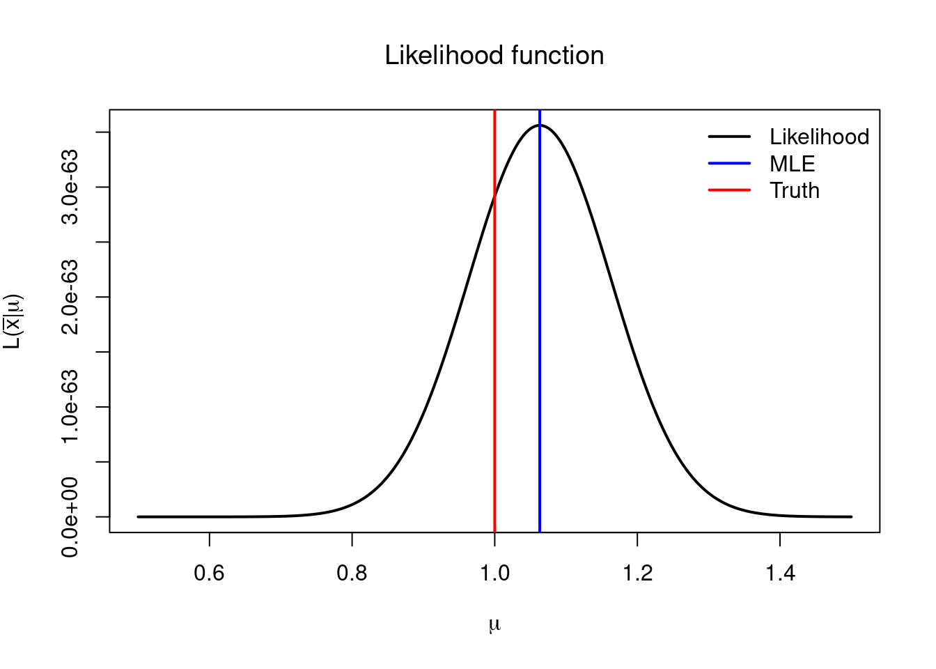
We now compare the distribution estimated through the MLE (\(\hat{\mu}\)) against the observed (empirical) distribution of the data and the true density (\(\mu=1\)).
# Visualize estimated density VS normal densities under different mus
plot(density(data), xlim = c(-3,3), ylim = c(0,0.5), lwd = 3, xlab = "x", ylab = "density",
     main = "Density Comparison")
x <- seq(-2,4,length.out = 100)
mus <- seq(-2, 2, length.out = 5)
ignore <- mapply(lines, y = lapply(mus, dnorm, x = x, sd = 1),
       MoreArgs = list('x' = x, 'col' = "gray", 'lwd' = 1))
abline(v = mus, lwd = 1, col = "gray")
lines(x, dnorm(x, mean = 1, sd = 1), col = "red", lwd = 2)
abline(v = 1, lwd = 2, col = "red")
lines(x, dnorm(x, mean = mle, sd = 1), col = "blue", lwd = 2)
abline(v = mle, lwd = 2, col = "blue")
legend("left", bty = "n", legend = c("data", "mle", "truth"), col = c("black", "blue", "red"), lwd = 2)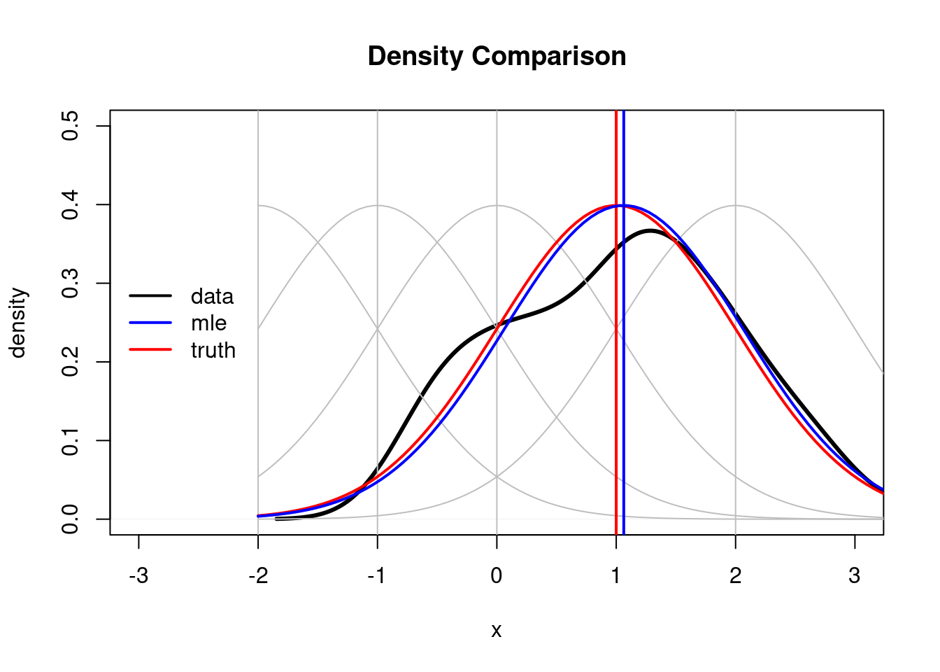
# Visualize estimated cdf VS normal cdfs under different mus
datacdf <- ecdf(data)
x <- seq(-3,3,length.out = 100)
plot(x = x, y = datacdf(x), xlim = c(-3,3), lwd = 2, xlab = "x", ylab = "CDF", main = "CDF comparison", type = "l")
mus <- seq(-2, 2, length.out = 10)
ignore <- mapply(lines, y = lapply(mus, pnorm, q = x, sd = 1),
       MoreArgs = list('x' = x, 'col' = "gray", 'lwd' = 1))
lines(x, pnorm(x, mean = 1, sd = 1), col = "red", lwd = 2)
lines(x, pnorm(x, mean = mle, sd = 1), col = "blue", lwd = 2)
legend("topleft", box.col = "white", legend = c("data", "mle", "truth"), col = c("black", "blue", "red"), lwd = 2)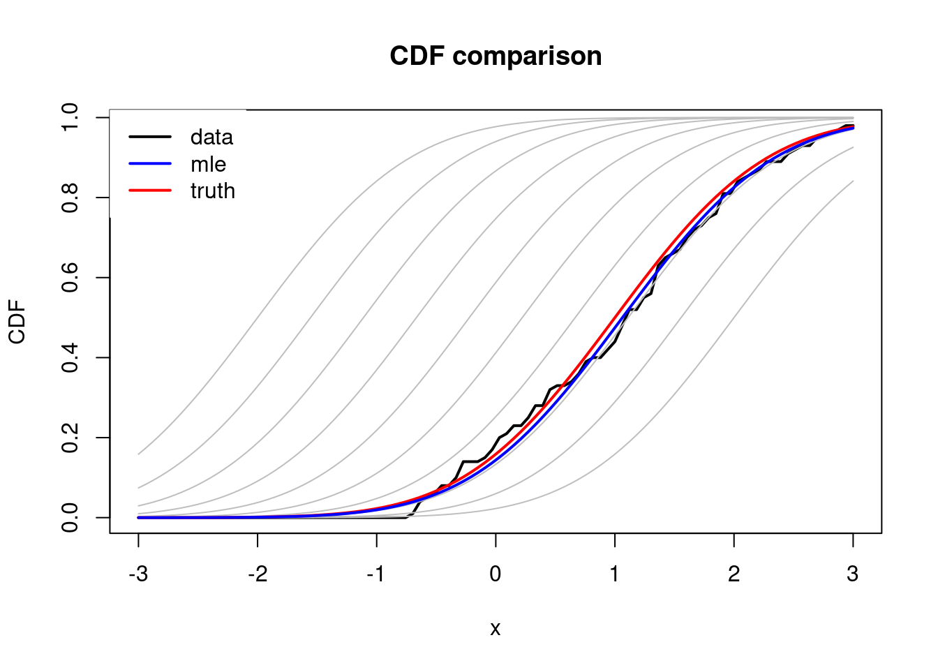
As discussed in Section 4.1 the value \(\bar{x}\) is typically equated with the experimentally observed data. However, in the probabilistic world \(\bar{x}\) is interpreted as just a ‘realization’ of the random vector \(\bar{X}\). Now observe that \(\hat{\theta}(\bar{x})\), the MLE for \(\theta\), is a function of \(\bar{x}\), and if we now think of \(\bar{x}\) as a realization of \(\bar{X}\), then in fact we may consider the random variable \(\hat{\theta}(\bar{X})\). Now, what does this mean in our statistical framework? Well, if a particular value \(\bar{x}\) is equated with the experimentally observed data, then we can think of the experiment as a probabilistic procedure that outputs a random value of \(\bar{x}\) every time it is performed, thus we think of the experiment as a sampling procedure of \(\bar{X}\) under its true distribution. Thus, the results of our estimation, in particular the value of the MLE point estimate, can also be seen as random (which makes sense since in reality if we repeated the experiment we wouldnt expect to obtain the same conclusions but not necessarily exactly the same results). The MLE then becomes a random variable and as such we may study its probabilistic behaviour, for example may study its variance \(\mathbb{Var}\left(\hat{\theta}(\bar{X})\right)\) which gives us a measure of how much we expect our estimation to vary if we repeated the experiment multiple times; and even more, we may study the probability that the MLE (or in general our statistical procedure) provides a good estimate for the real distribution of \(\bar{X}\), or the probability that it fails to do so. In the particular case of the MLE point estimate we may, for example, study the difference between \(\hat{\theta}(\bar{X})\) and the true value of \(\theta\).
# Generate 1000 random samples of size 100 each
mu <- 1 # set a true value of the parameter
datas <- matrix(rnorm(10000*100, mean = mu, sd = 1), nrow = 100)
# Compute MLE for each sample of size 100
mles <- colMeans(datas)
# Visualize MLE density and compare with true value mu0
# Estimated density
plot(density(mles), lwd = 2, xlab = TeX("$\\hat{\\mu}(\\bar{x})$"), ylab = "Density", main = TeX("MLE ($\\hat{\\mu}(\\bar{X})$) density"))
# True density
x <- seq(-0.7, 1.5, length.out = 1000)
lines(x = x, y = dnorm(x, mean = mu, sd = sqrt(1/100)), lwd = 2, col = "red")
legend("topleft", legend = c("MLE sample density", "MLE true density"), col = c("black", "red"), lwd = 2, bty = "n")
abline(v = mean(mles), col = "blue", lwd = 2)
abline(v = mu, col = "black", lwd = 2)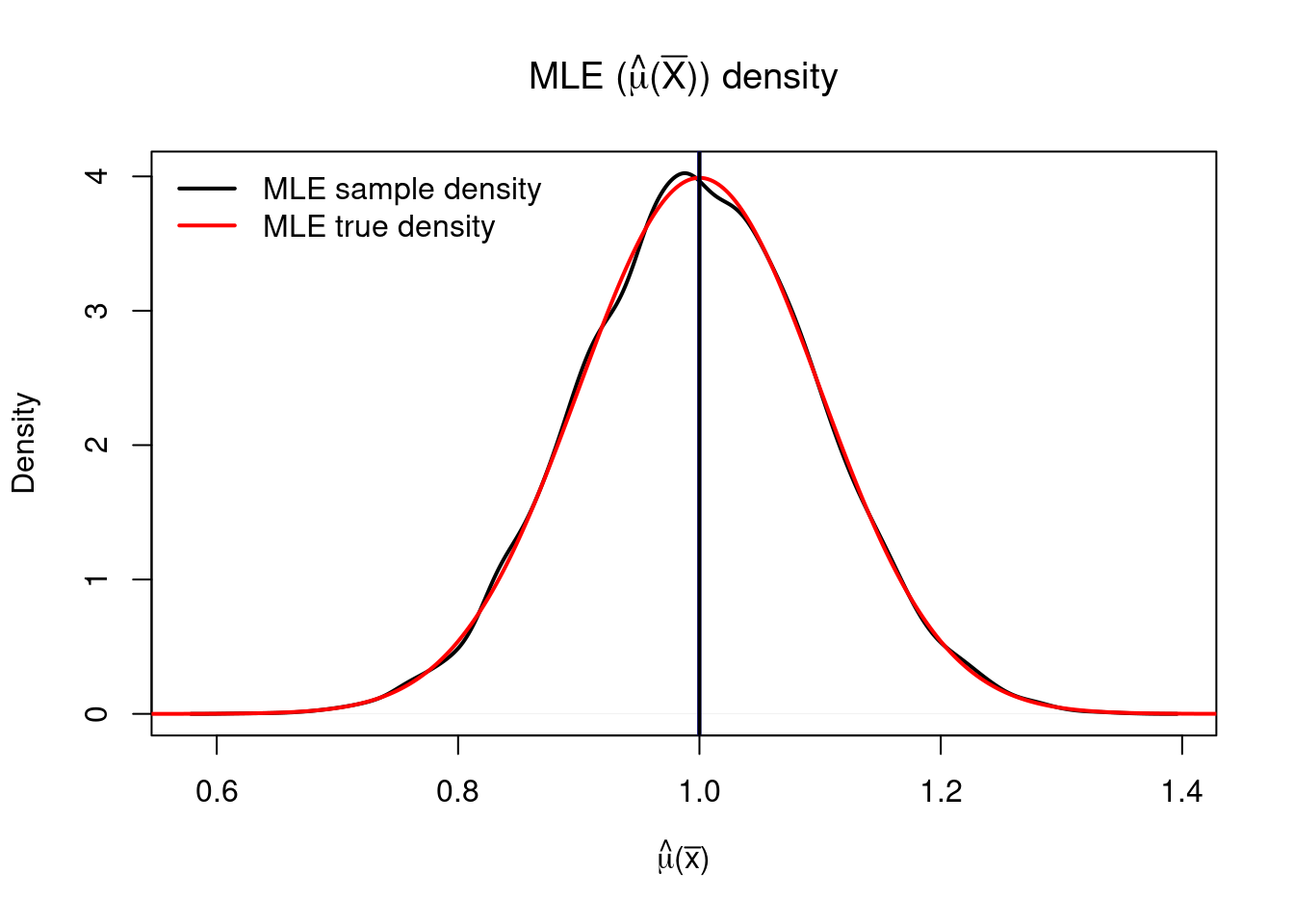
Thus, for example, we may compute the probability that \(\left\lvert \hat{\mu}(\bar{X}) - \mu \right\rvert> a\) given that \(\bar{X}\overset{i.i.d}\sim normal(\mu,1)\) (i.e. under the model \(\mathcal{P}_\mu\)), we have
\[\begin{align} \mathbb{P}_\mu\left(\left\lvert \hat{\mu}(\bar{X}) - \mu \right\rvert> a\right) &= 1-\int_{\mu-a}^{\mu+a} \sqrt{\frac{n}{2\pi}} e^{-\frac{n(x - \mu )^2}{2}} dx \\ &=1- \int_{-a}^a \sqrt{\frac{n}{2\pi}} e^{-\frac{n x^2}{2}}dx; \end{align}\] observe that in this case the distribution of the distance between the estimator \(\hat{\mu}(\bar{X})\) and \(\mu\) under \(\mathcal{P}_{\mu}\) has distribution \(normal(0,1/n)\) which does not depend on \(\mu\) so that we can assure, irrespectively of the value of \(\mu\), that the distance of our estimator \(\hat{\mu}(\bar{x})\) and \(\mu\) will always be less than \(a\) with probability6
\[ \int_{-a}^a \sqrt{\frac{n}{2\pi}} e^{-\frac{n x^2}{2}}dx. \]
4.3 Hypothesis testing
4.3.1 Definition, Evaluation, and Power
Based on (Casella and Berger 2002, sec. 8.1) for the definition of hypothesis, and (Casella and Berger 2002, sec. 8.3.1) for their evaluation and the power function.
The goal of a hypothesis test is to decide, based on a sample from the population, which of two complementary hypothesis is true.
Definition 4.5 (Hypothesis Test) A hypothesis testing procedure is a rule that sepecifies:
- For which sample values \(\bar{x}\in\mathbb{R}^n\) the decision is made to accept \(H_0\) as true.
- For which sample values \(\bar{x}\in\mathbb{R}^n\) the decision is made to reject \(H_0\) (‘in acceptance of \(H_1\)’).
Typically a hypothesis test is specified in terms of a test statistic \(W(X_1,\dots,X_n)\), i.e. a function \(W\colon \mathbb{R}^n\to\mathbb{R}\) of the sample \(\bar{X}=(X_1,\dots,X_n)\).
Example 4.6 (Normal \(\sigma\) known) Let \(X_1,\dots,X_n\) be an i.i.d sample of a \(normal(\mu,\sigma)\) distribution with unknown \(\mu\) and known \(\sigma\). Recall from Example 4.4 that the MLE for \(\mu\) is \[ \hat{\mu}(\bar{X})=\tilde{X}. \] Fix a value \(\mu_0\). We may define a decision rule for testing \(H_0\colon\mu=\mu_0\) versus \(H_1\colon\mu\neq \mu_0\) using the statistic \(\hat{\mu}(\bar{X})\). To do so it would be reasonable to consider a rejection region of the form
\[ \begin{aligned} R&=\{\bar{x}\in\mathbb{R}^n\colon\left\lvert \hat{\mu}(\bar{x}) - \mu_0 \right\rvert > c_n\}\\ &=\{\bar{x}\in\mathbb{R}^n\colon\left\lvert \tilde{x} - \mu_0 \right\rvert > c_n\}\subset \mathbb{R}^n. \end{aligned} \]
for some prespecified value of \(c_n\),7.8Definition 4.6 (Type I and II Errors) A hypothesis test for \(H_0\colon \theta\in\Theta_0\) VS \(H_1\colon \theta\not\in\Theta_0\) can make two types of errors
- Type I error: When \(H_0\colon\theta\in\Theta_0\) is true but the test decides that \(H_0\) is false (false positive).
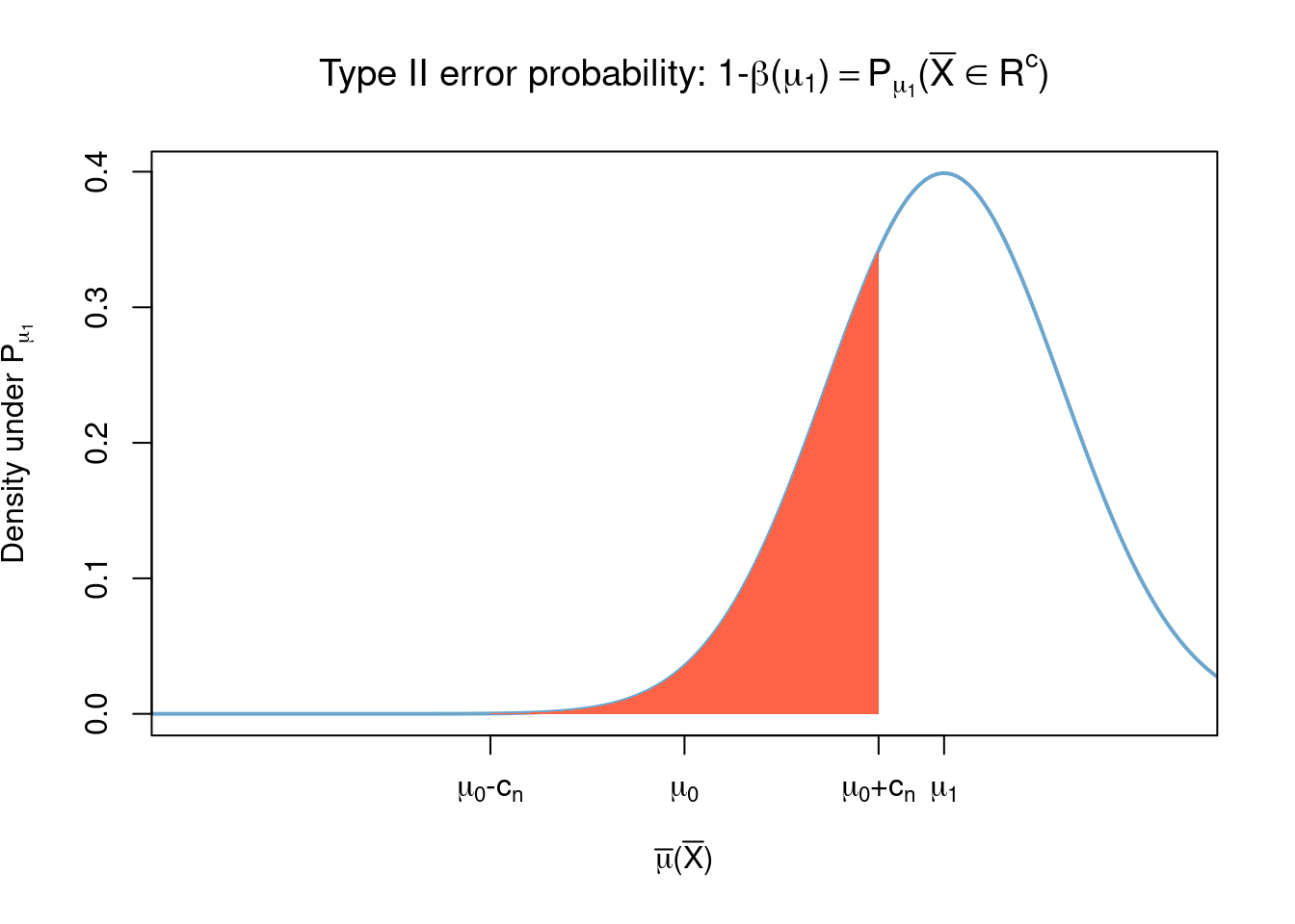
- Type II error: When \(H_1\colon\theta\not\in\Theta_0\) is true but the test decides that \(H_0\) is true (false negative).
| Decision | |||
|---|---|---|---|
| Accept H_0 | Reject H_0 | ||
| Truth | H_0 | Correct Decision | Type I error |
| H_1 | Type II error | Correct Decision |
Now let \(\theta\in\Theta_0\) and assume \(\bar{X}\sim \mathcal{P}_\theta\) (i.e. assume \(\theta\) is the true value of the parameter) so that the test will make a mistake, a Type I error, if \(\bar{X}\in R\) which occurs with probability9
\[\mathbb{P}_\theta(\bar{X}\in R).\] Alternatively, if \(\theta\in \Theta_0^c\) and we assume \(\bar{X}\sim \mathcal{P}_\theta\) then the test will make a mistake, a Type II error, if \(\bar{X}\in R^c\) which occurs with probability \[1-\mathbb{P}_\theta(\bar{X}\in R).\] Observe then that the function \[\theta\mapsto \mathbb{P}_\theta(\bar{X}\in R)\] summarizes all the information of the test with rejection region \(R\), in particular summarizes the probabilities of making Type I and II errors, thus calling for the following definition.
Note that
- For \(\theta\in\Theta_0\), \(\mathbb{P}_\theta(\text{Type I error}) = \beta(\theta)\)
- For \(\theta\in\Theta_1\), \(\mathbb{P}_\theta(\text{Type II error}) = 1-\beta(\theta)\),
thus, the ideal power function is \(0\) for all \(\theta\in\Theta_0\), since this would mean that Type I errors occur with zero probability, and \(1\) for all \(\theta\in\Theta_0^c\), since this would mean that Type II errors occur with zero probability.
Example 4.7 (Two-Sided Z-test) Recall the test \(H_0\colon\mu=\mu_0\) VS \(H_1\colon\mu\neq\mu_0\) of Example 4.6 with rejection region \[ R=\{\bar{x}\in\mathbb{R}^n\colon\left\lvert \tilde{x} - \mu_0 \right\rvert > c_n\}. \]
Observe that the test will make a Type I error if \(\mu_0\) is the true value of \(\mu\) and \(\left\lvert \tilde{X} - \mu_0 \right\rvert > c_n\), which occurs with probability (see Example 4.5) \[\beta(\mu_0) = \mathbb{P}_{\mu_0}(\left\lvert \tilde{X} - \mu_0 \right\rvert > c_n)= 1- \int_{\mu_0-c_n}^{\mu_0+c_n} \sqrt{\frac{n}{2\pi}} e^{-\frac{n(x - \mu_0 )^2}{2}} dx.\]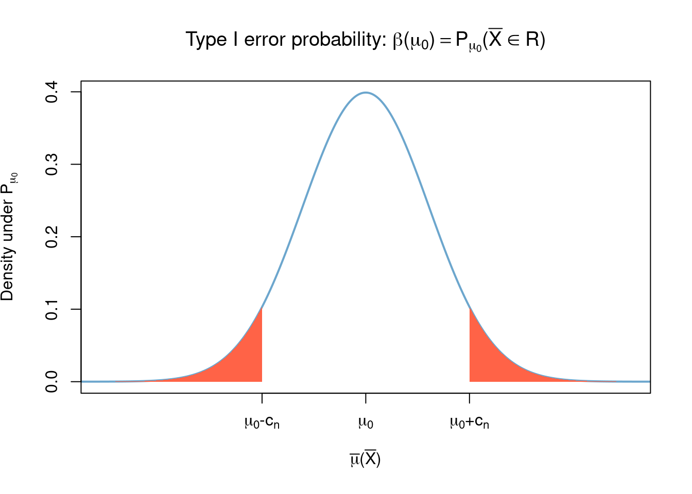
On the other hand, the test will make a Type II error if \(\mu_1\neq\mu_0\) is the true value of \(\mu\) and \(\left\lvert \tilde{X} - \mu_0 \right\rvert \leq c_n\), which occurs with probability \[ \begin{aligned} 1-\beta(\mu_1) = \mathbb{P}_{\mu_1}(\left\lvert \tilde{X} - \mu_0 \right\rvert \leq c_n)&= \mathbb{P}_{\mu_1}(\left\lvert \tilde{X} - \mu_0 \right\rvert > c_n)\\ &=\int_{\mu_0-c_n}^{\mu_0+c_n} \sqrt{\frac{n}{2\pi}} e^{-\frac{n(x - \mu_1 )^2}{2}} dx. \end{aligned} \]
The power function of this test is \[ \begin{aligned} \beta(\mu) = \mathbb{P}_{\mu}(\left\lvert \tilde{X} - \mu_0 \right\rvert > c_n)= 1 - \int_{\mu_0-c_n}^{\mu_0+c_n} \sqrt{\frac{n}{2\pi}} e^{-\frac{n(x - \mu)^2}{2}} dx. \end{aligned} \] Now assume we choose \(c_n=c\sigma\sqrt{1/n}\) for some \(c>0\)10 so that, rearranging terms, the rejection region becomes
\[\begin{align} R &=\left\{\bar{x}\in\mathbb{R}^n\colon\left\lvert \frac{\tilde{x} - \mu_0}{\sigma/\sqrt{n}} \right\rvert > c\right\}\tag{4.1}\\ &=\left\{\bar{x}\in\mathbb{R}^n\colon \frac{\tilde{x} - \mu}{\sigma/\sqrt{n}} < - c + \frac{\mu_0 - \mu}{\sigma/\sqrt{n}} \right\}\cup \left\{\bar{x}\in\mathbb{R}^n\colon \frac{\tilde{x} - \mu}{\sigma/\sqrt{n}} > c + \frac{\mu_0 - \mu}{\sigma/\sqrt{n}}\right\}. \end{align}\]
Observe that when \(\bar{X}\overset{i.i.d}{\sim}normal(\mu,\sigma)\), i.e. under the assumption that the true value of the parameter is \(\mu\), we have that the random variable \[ Z(\bar{x}):=\frac{\tilde{x} - \mu}{\sigma/\sqrt{n}} \] (often called the Z-statistic) is \(normal(0,1)\) distributed (observe that its distribution does not depend on \(\mu\) nor \(\sigma\), nor \(n\)), so that the power function becomes11 \[ \begin{aligned} \beta(\mu)&=\mathbb{P}_\mu(\bar{X}\in R) \\ &=\mathbb{P}\left( Z(\bar{X}) \in \left[\frac{\mu_0 - \mu}{\sigma/\sqrt{n}} -c, \frac{\mu_0 - \mu}{\sigma/\sqrt{n}} +c\right]^c\right) \\ &= \mathbb{P}\left(\left\lvert Z+ \frac{\mu - \mu_0}{\sigma/\sqrt{n}} \right\rvert > c\right)\\ &=\frac{1}{\sqrt{2\pi}} \int_{-\infty}^{\frac{\mu_0 - \mu}{\sigma/\sqrt{n}} -c} e^{-\frac{x^2}{2}}dx + \frac{1}{\sqrt{2\pi}} \int_{\frac{\mu_0 - \mu}{\sigma/\sqrt{n}} +c}^\infty e^{-\frac{x^2}{2}}dx . \end{aligned} \]
where \(Z\) is a standard normal random variable.
```
Example 4.8 (Two-sided T-test) We now consider a hypothesis test of the form \(H_0\colon\mu = \mu_0\) VS \(H_1\colon\mu\neq\mu_0\) for a sample \(\bar{X}\) with \(normal(\mu,\sigma)\) distribution where both \(\mu\) and \(\sigma\) are unkown (\(\sigma\) is a nuissance parameter). Again it is reasonable to construct the rejection region \(R\) as
\[\begin{align} R &=\left\{\bar{x}\in\mathbb{R}^n\colon\left\lvert \frac{\tilde{x} - \mu_0}{S(\bar{x})/\sqrt{n}} \right\rvert > c\right\}\tag{4.2}\\ &=\left\{\bar{x}\in\mathbb{R}^n\colon \frac{\tilde{x} - \mu}{S(\bar{x})/\sqrt{n}} < - c + \frac{\mu_0 - \mu}{S(\bar{x})/\sqrt{n}} \right\}\cup \left\{\bar{x}\in\mathbb{R}^n\colon \frac{\tilde{x} - \mu}{S(\bar{x})/\sqrt{n}} > c + \frac{\mu_0 - \mu}{S(\bar{x})/\sqrt{n}}\right\}. \end{align}\]
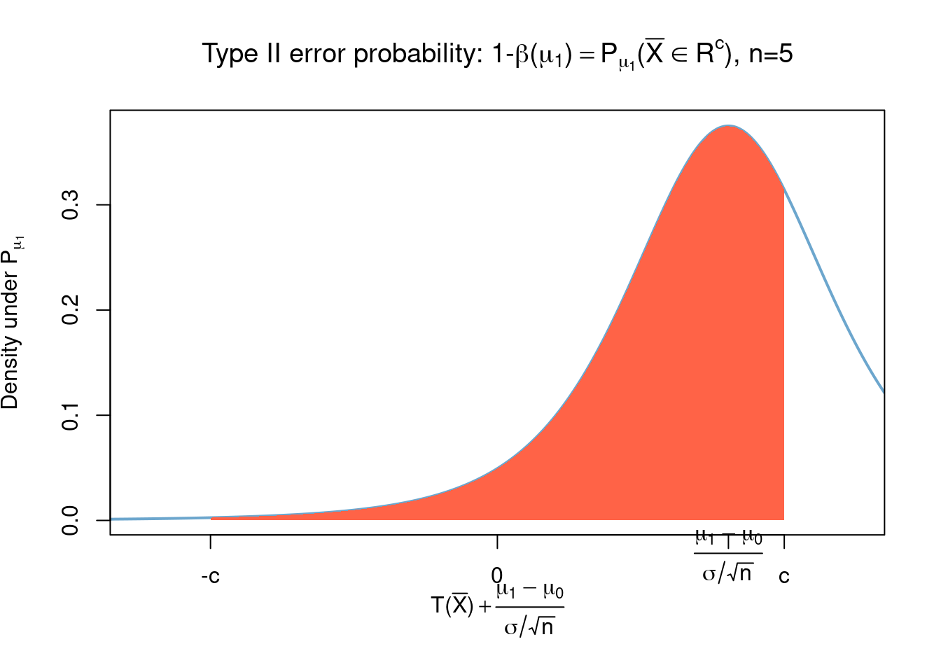
for some \(c>0\), where \(S^2\) is the sample variance \[ S^2(\bar{x}) = \frac{1}{n} \sum_{i=1}^n (x_i - \tilde{x})^2 \] which is also the MLE estimator for \(\sigma\). Letting \[ T :=\frac{\tilde{x} - \mu}{S(\bar{x})/\sqrt{n}} \] (called the \(T\)-statistic) we obtain that, under the model \(\bar{X}\overset{i.i.d}{\sim}normal(\mu,\sigma)\), \(T\) has Students-t distribution with \(n-1\) degrees of freedom (see Section 3.8 and also observe that its distribution no longer depends on \(\mu\) nor on \(\sigma\) but does depend on the sample size \(n\)) and the corresponding power function \(\beta(\mu)\) is given by12 \[\begin{align} \beta(\mu)&=\mathbb{P}_\mu(\bar{X}\in R) \\ &=\mathbb{P}\left( T(\bar{X}) \in \left[-c + \frac{\mu_0 - \mu}{S(\bar{X})/\sqrt{n}}, c + \frac{\mu_0 - \mu}{S(\bar{X})/\sqrt{n}}\right]^c\right)\\ &=\mathbb{P}\left(\left\lvert T(\bar{X}) + \frac{\mu - \mu_0}{S(\bar{X})/\sqrt{n}} \right\rvert > c\right) \end{align}\]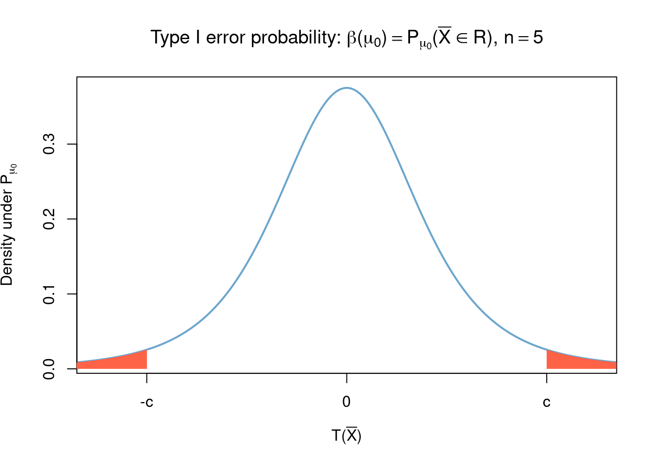
Definition 4.8
For \(0\leq\alpha\leq 1\), a test with power function \(\beta(\theta)\) is a size \(\alpha\) test if \[ \sup_{\theta\in\Theta_0} \beta(\theta)= \alpha. \]
- For \(0\leq\alpha\leq 1\), a test with power function \(\beta(\theta)\) is a level \(\alpha\) test if \[ \sup_{\theta\in\Theta_0} \beta(\theta)\leq \alpha. \]
Observe from the above definitions that a size (resp. level) \(\alpha\) test makes a Type I error with probability exactly (resp. less than) \(\alpha\), so that knowing the size of a test informs us about its Type I error probabilities but tells us nothing about the Type II error probabilities. Typically experimenters set their hypothesis in such a way that not making a Type I error is more important than not making a Type II error (or that making a Type II error is preferred over making a Type I error), then experimenters choose an \(\alpha\in (0,1)\) which is a ‘tolerable’ probability of making a Type I error, and finally (when possbile) choose an appripropiate sample size \(n\) to also control the Type II error probability.
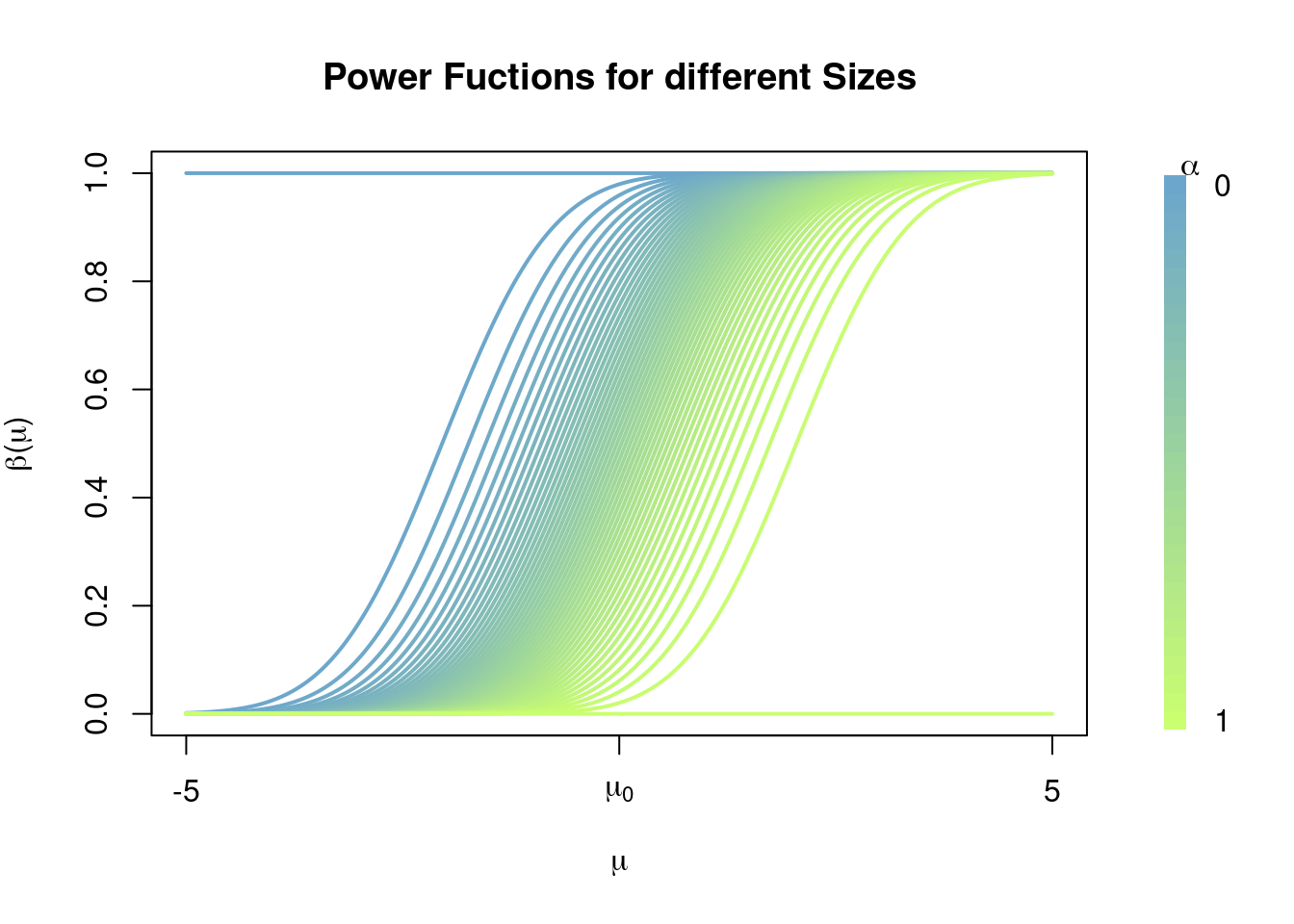
Each line in the graph above corresponds to the power function of a test with rejection region \[ R_\alpha=\left\{\bar{x}\in\mathbb{R}^n\colon \frac{\tilde{x} - \mu_0}{\sigma/\sqrt{n}} > c_\alpha\right\} \] where \(c_\alpha\) is chosen so that \[ \sup_{\mu\leq \mu_0} \beta(\mu) = \mathbb{P}\left(Z > c_\alpha\right) \leq \alpha; \] i.e. for each value of \(\alpha\) we find an appropriate constant \(c_\alpha\) such that the resulting test with rejection \(R_\alpha\) is a \(\alpha\)-level test, so that the probability of making a Type I error is assured to be less than \(\alpha\) irrespective of the value of \(\mu\).
Note how, for any non-trivial value of \(\alpha\), the function \(\beta(\mu)\) tends to \(0\) for \(\mu\leq\mu_0\), so that \(\mathbb{P}_\mu(\text{Type I error})=\beta(\mu)\) tends to zero as \(\mu\to-\infty\), and tends to 1 for \(\mu>\mu_0\), so that \(\mathbb{P}_\mu(\text{Type II error})=1-\beta(\mu)\) tends to zero as \(\mu\to\infty\). Note that this shape is consisten across different choices of \(\alpha\), but that for small \(\alpha\) the maximum value of \(1-\beta(\mu)\) in the range \((\mu_0,\infty]\) is larger than the corresponding maximum value for large choices of \(\alpha\), this is saying that having a tight control over Type I error probabilities (i.e. small choices of \(\alpha\)) comes with the cost of allowing for large Type II error probabilities \((1-\beta(\mu))\); and vice versa, large values of \(\alpha\) allow for larger values of \(\beta(\mu)\) on the range \((-\infty, \mu_0]\) thus allowing for larger Type I error probabilities, but with the gain of allowing smaller values of \(1-\beta(\mu)\), i.e. smaller Type II error probabilities.
What would you expect to be the shape of \(\beta(\mu)\) if we were proving the hypothesis \(H_0\colon\mu\geq \mu_0\) VS \(H_1\colon\mu<\mu_0\) instead, and for the hypothesis \(H_0\colon\mu = \mu_0\) VS \(H_1\colon\mu\neq\mu_0\)?
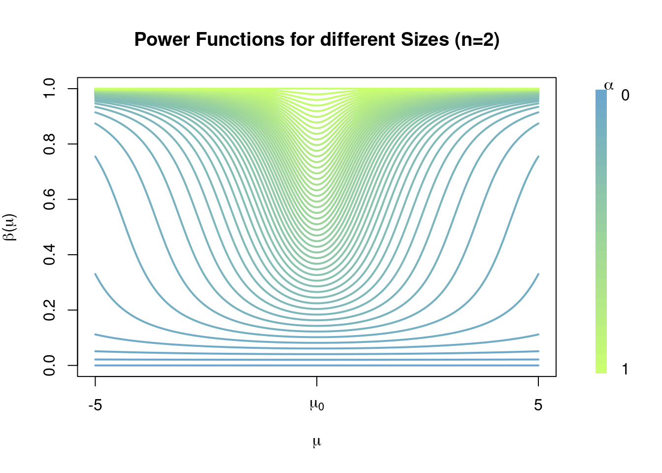
Observe how \(\beta(\mu)\) has the correct shape, how when \(\mu=\mu_0\) we have that \(\mathbb{P}_{\mu}(\text{Type I error})=\beta(\mu)\) is close to 0, whereas for \(\mu\neq\mu_0\) we have that \(\mathbb{P}_{\mu}(\text{Type II error})=1-\beta(\mu_0)\) is close to 0, and in fact becomes increasingly closer to \(0\) as \(\left\lvert \mu-\mu_0 \right\rvert\) becomes larger. Again note how this behaviour is consistent along different choices of the level \(\alpha\), and of course when \(\alpha\) is small we allow for smaller Type I error probabilities but larger Type II error probabilities, whereas for large \(\alpha\) we allow for smaller Type II error probabilities but large Type I error probabilities.
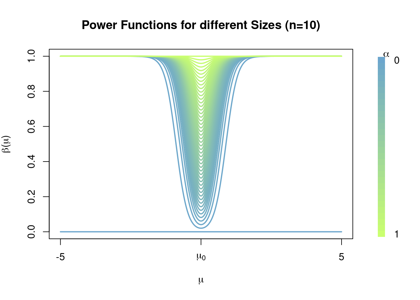
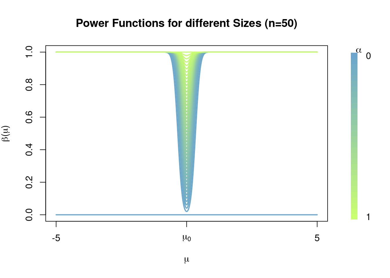
Observe how increasing the sample size \(n\) allows for the construction of level \(\alpha\) tests with lower Type II error probabilities, see how the power function becomes close to 1 for values away from \(\mu_0\) and that this is ‘faster’ when \(n=5\) than when \(n=2\); i.e. the power functions for tests with sample size \(n=5\) ‘are better’ than those with sample size \(n=2\). For \(n=50\) we have
4.3.2 p-Values
Based on (Casella and Berger 2002, sec. 8.3.4), specifically Def. 8.3.26, Thm. 8.3.27, and Exms. 8.3.28 and 8.3.29.
After a hypothesis test is done, results must be reported in a statistically meaningful way. One method is to simply report the size \(\alpha\) of the test. If \(\alpha\) is small, the decision to reject \(H_0\) is fairly convincing. A p-value \(p(\bar{X})\) reports the results of a test in a more continuous scale, rather than just the dichotomous decision to ‘Accept \(H_0\)’ or to ‘Reject \(H_0\)’. An advantage of reporting a p-value is that each reader can choose the \(\alpha\) that he considers appropriate (typical choices are 0.001, 0.01, and 0.05) and then compare the reported \(p(\bar{x})\) with \(\alpha\) to know whether this data support rejection of \(H_0\).
Note that, for every \(0\leq \alpha \leq 1\), a test with rejection region \[ R=\{\bar{x}\colon p(\bar{x})\leq\alpha\} \] is a level \(\alpha\) test based on \(p(\bar{X})\) so that, as mentioned before, each reader can choose his own \(\alpha\) and determine whether or not the data support rejection of \(H_0\). Thus, in practice, the easiest way to interpret a p-value \(p(\bar{x})\) is by saying that if we decide to reject the null hypothesis \(H_0\) based on the value of \(p(\bar{x})\) then we would incur in a Type I error with probability at most \(p(\bar{x})\) (thus small values of \(p(\bar{x})\) support rejection of \(H_0\) while for large values of \(p(\bar{x})\) rejection of \(H_0\) becomes increasingly dubious), this is achieved if the experimenter decided to choose \(\alpha=p(\bar{x})\). Again note that the p-value tells us nothing about Type II error probabilities which have to be controlled through other means, usually by determining an appropriate sample size \(n\).
The following theorem gives the typical way in which p-values are constructed.
Example 4.11 (One-sided Z-test p-value) Recall the test of \(H_0\colon \mu\leq\mu_0\) VS \(H_1\colon\mu>\mu_0\) in Example 4.9. Note that
large values of
\[Z(\bar{x})=\frac{\tilde{x}-\mu_0}{\sigma/\sqrt{n}}\]
(the Z-statistic) support rejection of \(H_0\). Thus, by Theorem 4.1,
the statistic
\[
p(\bar{x}) = \sup_{\mu\leq\mu_0} \mathbb{P}_\mu( Z(\bar{X}) > Z(\bar{x}))
\]
is a valid p-value. We now show that
\[
\sup_{\mu\leq\mu_0} \mathbb{P}_\mu( Z(\bar{X}) > Z(\bar{x})) = \mathbb{P}_{\mu_0}(Z(\bar{X}) > Z(\bar{x})).
\]
Indeed, note that for every \(\mu\)
\[\begin{align}
\mathbb{P}_\mu( Z(\bar{X}) > Z(\bar{x}))
&= \mathbb{P}_\mu\left( \frac{\tilde{X}-\mu_0}{\sigma/\sqrt{n}} > Z(\bar{x})\right)\\
&= \mathbb{P}_\mu\left(\frac{\tilde{X}-\mu}{\sigma/\sqrt{n}} > Z(\bar{x}) + \frac{\mu-\mu_0}{\sigma/\sqrt{n}}\right)\\
&= \mathbb{P}_\mu\left(Z > Z(\bar{x}) + \frac{\mu-\mu_0}{\sigma/\sqrt{n}}\right)
\end{align}\]
where \(Z\) is an standard normal variable so that, in particular, its distribution does not depend on \(\mu,\sigma\) nor \(n\).
It follows that \[\begin{align} p(\bar{x})&=\sup_{\mu\leq\mu_0} \mathbb{P}_\mu( Z(\bar{X}) > Z(\bar{x}))\\ &= \sup_{\mu\leq\mu_0} \mathbb{P}_\mu\left(Z > Z(\bar{x}) + \frac{\mu-\mu_0}{\sigma/\sqrt{n}}\right) \\ &= \mathbb{P}(Z > Z(\bar{x})). \end{align}\]
Thus the p-value \(p(\bar{X})\) is given by \[\begin{align} p(\bar{X})&=\mathbb{P}\left(Z\geq Z(\bar{X})\right) %&= \P\(\frac{Z\sigma}{\sqrt{n}} + \mu_0 \geq \tilde{x}\) \end{align}\] where \(Z\) is a standard normal random variable independent of \(\bar{X}\).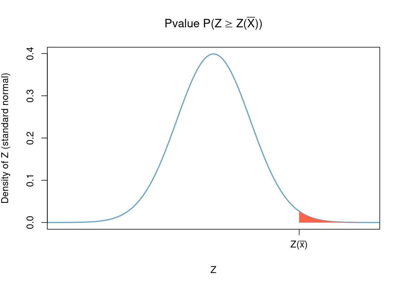
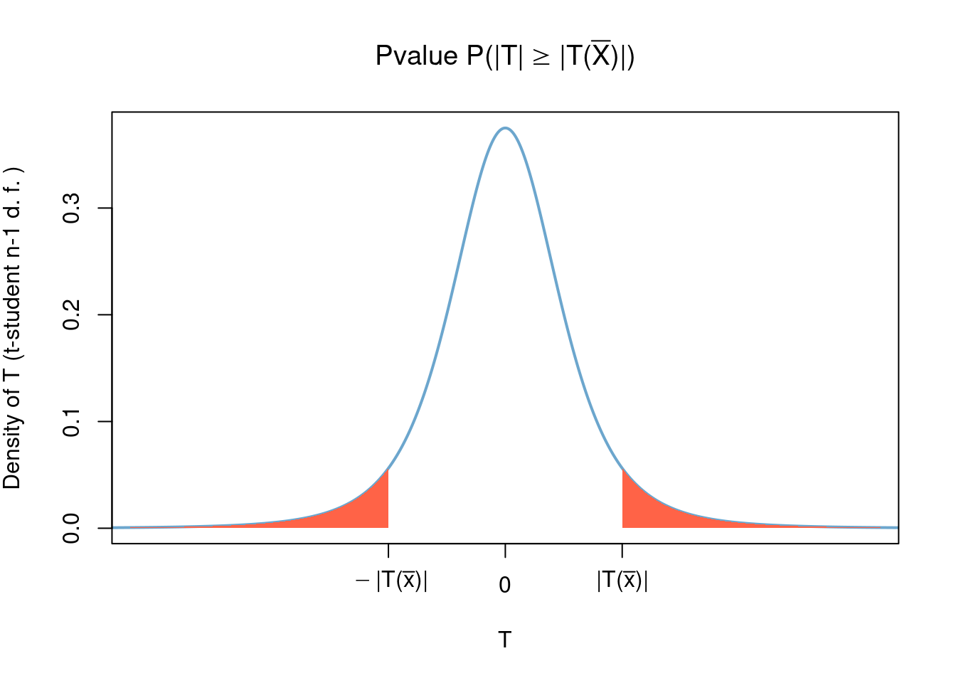
the statistic \[\begin{align} p(\bar{x}) &= \sup_{\mu\in\{\mu_0\}} \mathbb{P}_\mu( \left\lvert T(\bar{X}) \right\rvert > \left\lvert T(\bar{x}) \right\rvert)\\ &= \mathbb{P}( \left\lvert T \right\rvert > \left\lvert T(\bar{x}) \right\rvert) \end{align}\] is a valid p-value; here \(T\) is students-t distributed with \(n-1\) degrees of freedom. Of course, by the symmetry of \(T\), in this case we have \[\begin{align} p(\bar{X}) &= \mathbb{P}( \left\lvert T \right\rvert > \left\lvert T(\bar{X}) \right\rvert)\\ &= 2\mathbb{P}( T > \left\lvert T(\bar{X}) \right\rvert). \end{align}\] where \(T\) is a Students-t with \(n-1\) degrees of freedom random variable that is independent of \(\bar{X}\).
4.3.3 Likelihood Ratio Tests (LRTs)
Based on (Casella and Berger 2002 Sec. 8.2.1), specifically Def. 8.2.1, Exms. 8.2.2 and 8.2.6.
In this section we introduce a general theoretical framework for the construction of the rejection region \(R\) which can be applied to any parameter \(\theta\) of any model \(\mathcal{P}_\theta\).
Example 4.13 (Two-sided Z-test as LRT) Let \(\bar{X}=(X_1,\dots,X_n)\) be an i.i.d sample with \(normal(\mu,1)\) distribution. Consider testing \(H_0\colon \mu=\mu_0\) VS \(H_1\colon\mu\neq\mu_0\) (\(\mu_0\) is a number fixed by the experimenter prior to the experiment). Then, recalling that the MLE for \(\mu\) is \(\hat{\mu}(\bar{X})=\tilde{X}\), \[ \lambda(\bar{x}) = \frac{(2\pi)^{-n/2}e^{-\sum_{i=1}^n \frac{(x_i-\mu_0)^2}{2}}} {(2\pi)^{-n/2}e^{-\sum_{i=1}^n \frac{(x_i-\tilde{x})^2}{2}}}, \] and since \[ \sum_{i=1}^n (x_i-\mu_0)^2 = n(\tilde{x}-\mu_0)^2 + \sum_{i=1}^n (x_i-\tilde{x})^2, \] the LRT statistic becomes \[ \lambda(\bar{x}) = e^{-\frac{n(\tilde{x}-\mu_0)^2}{2}}. \] A LRT rejects \(H_0\) for small values of \(\lambda(\bar{x})\), so that it has a rejection region of the form
\[ \begin{aligned} R&=\{\bar{x}\colon \lambda(\bar{x})\leq c\}\\ &=\left\{\bar{x}\colon \left\lvert \tilde{x}-\mu_0 \right\rvert\geq \sqrt{-2\log(c)/n}\right\} \end{aligned} \]
for some \(c\in[0,1]\). Compare this with (4.1) by observing that as \(c\) varies along \([0,1]\) the term \(-2\log(c)\) varies along \((0,\infty)\).
Example 4.14 (Two-Sided T-test as LRT) Let \(\bar{X}=(X_1,\dots,X_n)\) be an i.i.d sample with \(normal(\mu,\sigma)\) distribution where both \(\mu\) and \(\sigma\) are unkown and that we are interested in testing \(H_0\colon \mu\leq\mu_0\) VS \(H_1\colon\mu>\mu_0\) (so that \(\sigma\) is a nuisance parameter). Then
\[\begin{aligned} \lambda(\bar{x}) &= \frac{\sup_{\mu\leq\mu_0, \sigma\geq 0} L(\mu,\sigma^2 \vert \bar{x})} {\sup_{\mu\in\mathbb{R}, \sigma\geq 0} L(\mu,\sigma^2 \vert \bar{x})}\\ &=\frac{\sup_{\mu\leq\mu_0, \sigma\geq 0} L(\mu,\sigma^2 \vert \bar{x})} {L(\hat{\mu},\hat{\sigma}^2 \vert \bar{x})} \end{aligned}\] where of course \(\hat{\mu}\) and \(\hat{\sigma}^2=\frac{1}{n}\sum (x_i - \tilde{x})^2\) are the MLEs of \(\mu\) and \(\sigma^2\). In particular, if \(\hat{\mu}\leq\mu_0\) then \[ \sup_{\mu\leq\mu_0, \sigma\geq 0} L(\mu,\sigma^2 \vert \bar{x}) = L(\hat{\mu},\hat{\sigma}^2 \vert \bar{x}), \] and if \(\hat{\mu}>m_0\) then the restricted maximum is \(L(\mu_0, \hat{\sigma}^2_0\vert \bar{x})\) where \(\hat{\sigma}^2_0= \sum (x_i-\mu_0)^2/n\), so that \[ \lambda(\bar{x}) = \begin{cases} 1 & \text{ if }\hat{\mu} \leq \mu_0\\ \frac{L(\mu_0, \hat{\sigma}^2_0\vert \bar{x})}{L(\hat{\mu},\hat{\sigma}^2 \vert \bar{x})} & \text{ otherwise}. \end{cases} \] With some rearranging of the terms it can be shown that the test based on the statistic \(\lambda(\bar{X})\) is equivalent to a test based on the \(t\)-statistic \[ t=\frac{\tilde{X}-\mu}{\sqrt{\hat{\sigma}^2/n}}. \] which has Student’s-t distribution with \(n-1\) degrees of freedom.Here you can think of the call to \(rnorm\) as ‘performing an experiment’ that outputs some data \(\bar{x}\) under the true distribution of \(\bar{X}\sim normal(1,1)\). Of course, in contrast with the typical scenario in real life, in this case we do know the true distribution of the data since we are simulating it, this is useful if one wants to study how well does the statistical procedure works, for example by running the code multiple times (which you can think of as repeating the experiment multiple times) one can get a good estimate of the expected distance between \(\hat{\mu}(\bar{x})\) and the true parameter that we used for the simulations, in this case \(\mu=1\).↩
Here the intuition of thinking an experiment as a ‘machine’ generating values of \(\bar{x}\) under the true distribution of \(\bar{X}\) is equated in the code with a call to \(rnorm\). You can think of the columns of the matrix datas as multiple repetitions of the experiment, each with a different output value of \(\bar{x}\).↩
This can be used to construct what are called ‘Confidence intervals’ for \(\mu\) which are of the form \[ \left[\hat{\mu}(\bar{X}) - a, \hat{\mu}(\bar{X}) + a\right]; \] observe that this interval captures the true parameter \(\mu\) with probability \[ \int_{-a}^a \sqrt{\frac{n}{2\pi}} e^{-\frac{n x^2}{2}}dx. \]↩
Later on we will discuss good choices for \(c_n\)↩
At this point this hypothesis test, or decision rule, is intuitively reasonable but somehow arbitrary. Further ahead we will introduce Likelihood Ratio Tests which provide a general theoretical framework for the construction of rejection regions / hypothesis tests / decision rules; turns out that the decision rule of this example can be obtained as a LRT.↩
Here we use the notation \(\mathbb{P}_\theta\) for the distribution of \(\bar{X}\) under the assumption \(\bar{X}\sim\mathcal{P}_\theta\); i.e. assuming that the true model is \(\mathcal{P}_\theta\). Here we keep the same letter \(\theta\) since later on we will want to consider \(\theta\) as a variable (much in the same sense in which we consider \(\theta\) to be a variable in the definition of the likelihood function \(L(\bar{x}\vert \theta)\).↩
Further below we will argument how to choose \(c\) based on how big we want the Type I error probabilit to be.↩
Here again we have a connection with Confidence Intervals, in this case with the interval \[ \left[\frac{\mu_0 - \mu}{\sigma/\sqrt{n}} -c, \frac{\mu_0 - \mu}{\sigma/\sqrt{n}} +c\right]\].↩
Here again we have a connection with Confidence Intervals, in this case the interval \[ \left[\frac{\mu_0 - \mu}{S(\bar{x})/\sqrt{n}} -c, \frac{\mu_0 - \mu}{S(\bar{x})/\sqrt{n}} +c\right]\].↩
The above graph is not entirely illustrative, to ease computations we have plotted the density of \[ T(\bar{X}) + \frac{\mu_1 - \mu_0}{\sigma/\sqrt{n}} \] which, for large enough values of \(n\) approximates very well the distribution of \[ T(\bar{X}) + \frac{\mu_1 - \mu_0}{S(\bar{X})/\sqrt{n}} \] which is the one that truly interests us.↩